---
schema_version: 1
title: 'Gasoline Price Changes and Consumer Inflation Expectations: Experimental Evidence'
authors:
- Felix Aidala
- Olivier Armantier
- Gizem Koşar
- Jason Somerville
- Giorgio Topa
- Wilbert van der Klaauw
language: en
edition: Author manuscript
paper_url: https://jason-somerville.com/papers/gasoline-inflation-expectations/
pdf_url: https://jason-somerville.com/files/gasoline-inflation-expectations/paper.pdf
format: Markdown with TeX mathematics
---
# **Gasoline Price Changes and Consumer Inflation Expectations: Experimental Evidence**[^1]
Felix Aidala, Olivier Armantier, Gizem Koşar, Jason Somerville,\
Giorgio Topa and Wilbert van der Klaauw[^2]
## Abstract
Using an experimental approach, we show that inflation expectations respond to gasoline price fluctuations. The effect, however, is small compared to other goods (food, durable goods) and not disproportionately large relative to the expenditure share of gasoline in households’ basket. The effect also weakens with the forecast horizons and displays substantial asymmetry: inflation expectations respond significantly more to positive than negative gasoline price shocks. A counterfactual exercise suggests that while the sharp rise in gasoline prices that followed the Russian invasion of Ukraine contributed substantially to short-term inflation expectations dynamics, the subsequent decline in gasoline prices did not.
JEL Codes: C93, D84, E31, E37, E52, Q43 \
Keywords: Survey experiment, inflation expectations, gasoline prices, household survey\
## Introduction
Inflation expectations (IE hereafter) play a key role in macroeconomic models and monetary policy (see e.g. Mester (2022)). Understanding the factors that influence IE is therefore an important question that has attracted substantial attention (see e.g. D’Acunto et al. (2023)). In an influential paper, (Coibion and Gorodnichenko 2015) found that crude oil price fluctuations explain almost entirely the dynamics in consumers’ short-term IE between 2000 and 2013.[^3] The authors attribute this extreme sensitivity to the fact that gasoline prices are highly visible and salient to consumers. As documented below, this view has become prevalent among policy makers, the media and prominent economists. Recent evidence, however, has challenged the conventional view (see e.g. Binder (2018) or Kilian and Zhou (2023b)). Notably, (Kilian and Zhou 2022a) show that (Coibion and Gorodnichenko 2015)’s result is highly sensitive to the sample period, model specification and measure of gas prices (i.e. retail gasoline vs. crude oil). Using SVAR models, (Kilian and Zhou 2022a) find the contribution of gasoline prices to IE to be much weaker. In this paper, we add to the literature by proposing an alternative experimental method to measure the sensitivity of IE to gasoline price shocks, and by applying this method in May 2022, at the height of the sharp rise in gasoline prices that followed the Russian invasion of Ukraine.
The role gasoline prices play in the formation of consumers’ IE was extensively discussed when (nominal) gasoline prices rose to record levels after the 2022 Russian invasion of Ukraine. James Bullard, President of the Federal Reserve Bank of St. Louis stated in April 2022 “... *inflation expectations of households in particular is driven by some salient prices, in particular the gasoline prices. And so, one should watch out how the gasoline prices develop, because this might actually destabilize the inflation anchor*.”[^4] Similarly, Loretta Mester, President of the Federal Reserve Bank of Cleveland, noted in September 2022 that “*The rise in inflation expectations since last year has been concentrated in short-term expectations, which rose with the rise in gasoline and food prices. More recently, these short-term expectations have moved down with gasoline prices*.”[^5] Among notable academics, (Reis 2022) argued that “... *some of the relative prices that moved the most in 2021 (like gasoline prices or cars) were among those most visible to consumers, who will tend to overreact to them when forming their expectations*.” In July 2022, Paul Krugman wrote “*We know from long experience that one-year inflation expectations basically reflect the price of gasoline*.”[^6]
To explore whether these statements find empirical support, we measure the sensitivity of short- and medium-term IE to gasoline price shocks in May–June 2022. We do so using an experiment embedded in the Federal Reserve Bank of New York’s Survey of Consumer Expectations (SCE hereafter). The goal of the within-subject experiment is to evaluate the extent to which the IE of survey participants respond to exogenous and controlled hypothetical gasoline price shocks at a specific point in time. To benchmark our results, we conduct additional treatments with commensurate price shocks for food and durable goods, which also saw notable changes in 2021–2022.
In principle, the advantage of an experiment embedded in a survey is to enable causal identification through controlled exogenous variations. As discussed in section [3](#sec:Experiment), this approach has been successfully applied in a growing range of economic settings. For example, (Armantier et al. 2022) conducted a similar experiment with hypothetical inflation shocks to evaluate the extent to which long-term IE remain anchored. Beyond providing causal estimates, the approach allows us to measure whether IE respond to both positive and negative gasoline price changes in real-time, for instance, at the height of an actual gasoline price shock in our case. Moreover, because the experiment generates treatment effects at the individual level, we can study the heterogeneity in responses to gasoline price shocks across individuals. Then, we can use our estimates to conduct counterfactual exercises to gauge the relative role played by gasoline, food and durable good price changes in explaining the evolution of IE after the Russian invasion of Ukraine.
Our experimental results show a statistically significant impact of gasoline price shocks on short-term IE, consistent with existing evidence (e.g. Binder (2018), Kilian and Zhou (2022a, 2022b)). The we identify effect is more muted for longer-term IE and largely limited to *increases* in gasoline price inflation. Specifically, we estimate one- and three-year ahead IE to increase by 0.075 and 0.051 percentage point (pp hereafter) on average in response to a positive 1.0pp gasoline prices shock, respectively. In contrast, we estimate that one- and three-year ahead IE decline by 0.009pp and 0.001pp on average in response to a negative 1.0pp shock to gasoline prices, respectively.
These estimates can be expressed as elasticities defined as the percent change in (one- or three-year ahead) IE that results from a one percent increase in gasoline prices over the past year. The gasoline price elasticities of one-year and three-year IE is 0.55% and 0.45% for positive shocks and 0.04% and -0.01% for negative shocks, with the differences between positive and negative gasoline price shock elasticities being statistically significant.
The experiment also shows that IE are substantially more sensitive to food and durable good price shocks than to gasoline price shocks. Specifically, we find that a 1.0pp increase (decrease) in food prices is associated with an average change of +0.234pp (-0.130pp) in one-year ahead IE, and +0.203pp (-0.061pp) in three-year ahead IE. A 1.0pp increase (decrease) in durable good prices is associated with an average change of +0.180pp (-0.068pp) in year-ahead IE, and +0.149pp (-0.045pp) in three-year ahead IE. When benchmarked against their relative importance in household spending baskets, we find that respondents’ IE are not necessarily more sensitive to gasoline price increases. In particular, our results show IE to be relatively *less* sensitive to *declines* in gasoline price inflation when compared to *declines* in food or durable good price inflation.
To illustrate the contribution of gasoline, food and durable good price changes on IE dynamics, we consider the period following the February 2022 Russian invasion of Ukraine. A counterfactual simulation suggests that the sharp increase in gasoline prices that followed the invasion had a substantial impact on consumers’ IE, while the subsequent decrease in gasoline prices that started in July 2022 was mostly innocuous. The simulations also suggest that food price inflation played an almost equally important role on consumers’ IE, while durable good prices had little influence.
The paper is organized as follows. We describe in section [2](#sec:Data) the data and some empirical patterns linking gasoline price changes to IE dynamics. The experimental design is presented in section [3](#sec:Experiment). The results of the experiment for gasoline prices are discussed in section [4](#sec:SensitivityGas). We study heterogeneity in individual IE revisions in response to gasoline price shocks in section [5](#sec:Heterogeneity). The relative impact of food and durable good price shocks on IE is discussed in section [6](#sec:SensitivityOther). The results of the counterfactual simulation are reported in section [7](#sec:counterfactual). Finally, implications of our findings are discussed in section [8](#sec:Discuss).
## Data and Descriptive Evidence
### The Survey of Consumer Expectations
The data are from the [SCE](https://www.newyorkfed.org/microeconomics/sce), a monthly, nationally representative, internet-based survey with a rotating panel of approximately 1,300 household heads conducted by the Federal Reserve Bank of New York since June 2013. The SCE collects expectations and perceptions about a wide range of economic outcomes, both macroeconomic (e.g. inflation, home prices, unemployment), and at the personal level (e.g. income and spending growth, labor market outcomes, credit access).[^7] In addition to regular monthly surveys, the SCE occasionally fields “special surveys” on an ad-hoc basis to answer specific research or policy questions. The experiment described in section [3](#sec:Experiment) was part of such a special survey fielded in May and June 2022.
The SCE elicits different measures of IE. Below, we focus on short- and medium-term inflation point forecasts. The short-term horizon corresponds to the year-ahead rate of inflation (“Over the next 12 months”), while the medium-term horizon corresponds to three-year ahead rate of inflation, defined as the two-year ahead one-year rate of inflation (“Over the 12-month period between M+24 and M+36,” where M is the month in which the respondent takes the survey). For instance, a respondent taking the survey in May 2022 is asked about inflation “Over the 12-month period between May 2024 and May 2025.” For each horizon, the inflation forecasts are elicited in two steps. First, we ask respondents whether they think there will be inflation or deflation (defined as “the opposite of inflation”). Then, we ask what they think the rate (of inflation or deflation, depending on their previous response) will be over that horizon, expressed as a percent change.
### Descriptive Evidence
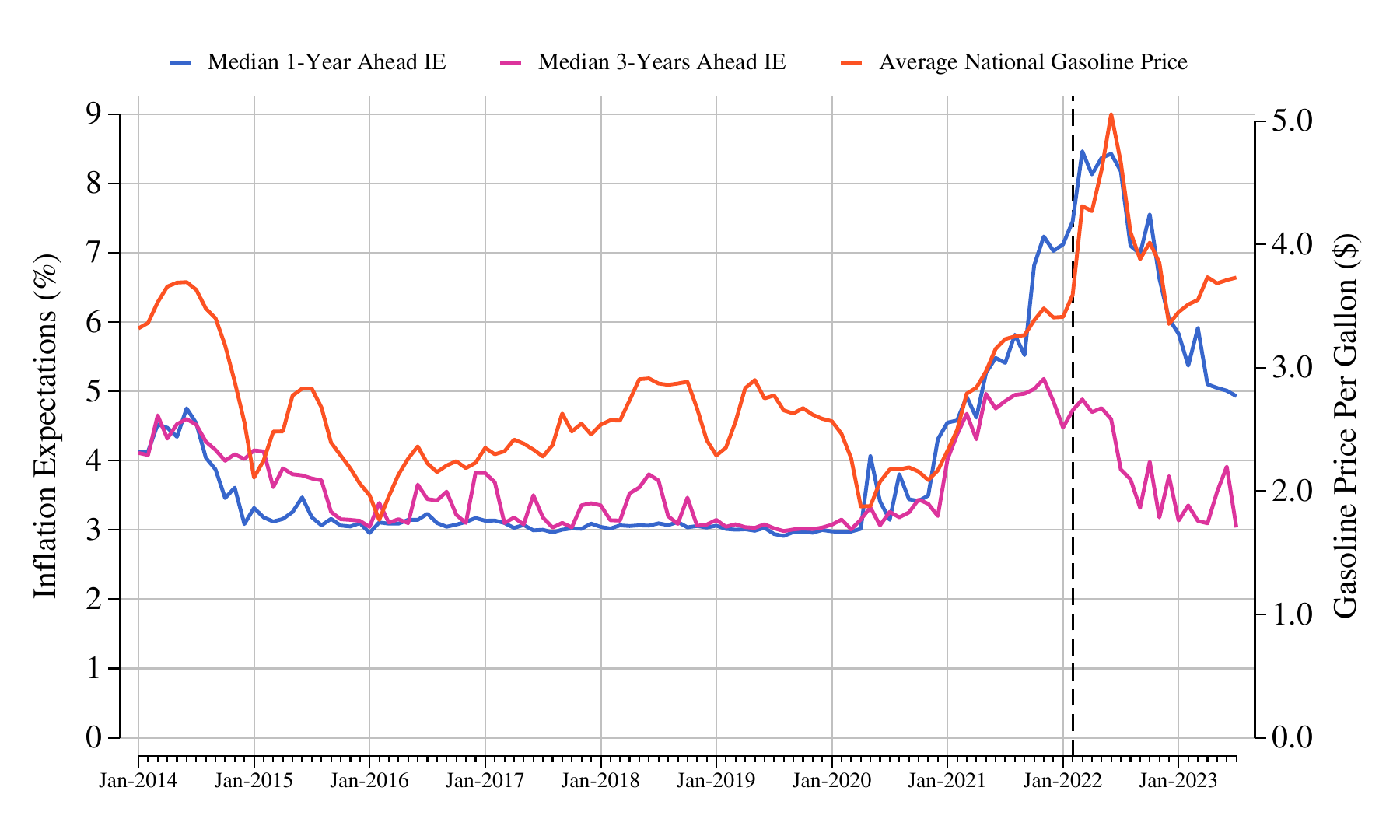
The blue and magenta lines in Figure [1](#fig:ie_gas_prices) show the median one- and three-year ahead IE between January 2014 and July 2023. The median one-year ahead IE rose sharply during the COVID-19 pandemic, from 3.0% in January 2020 to a series high of 8.5% in March 2022, after which it came down to 4.9% in July 2023. Changes in medium-term expectations have been more modest, with median three-year ahead IE rising from 3.1% in January 2020 to a peak of 5.2% in November 2021, and then declining to 3.0% in July 2023.[^8]
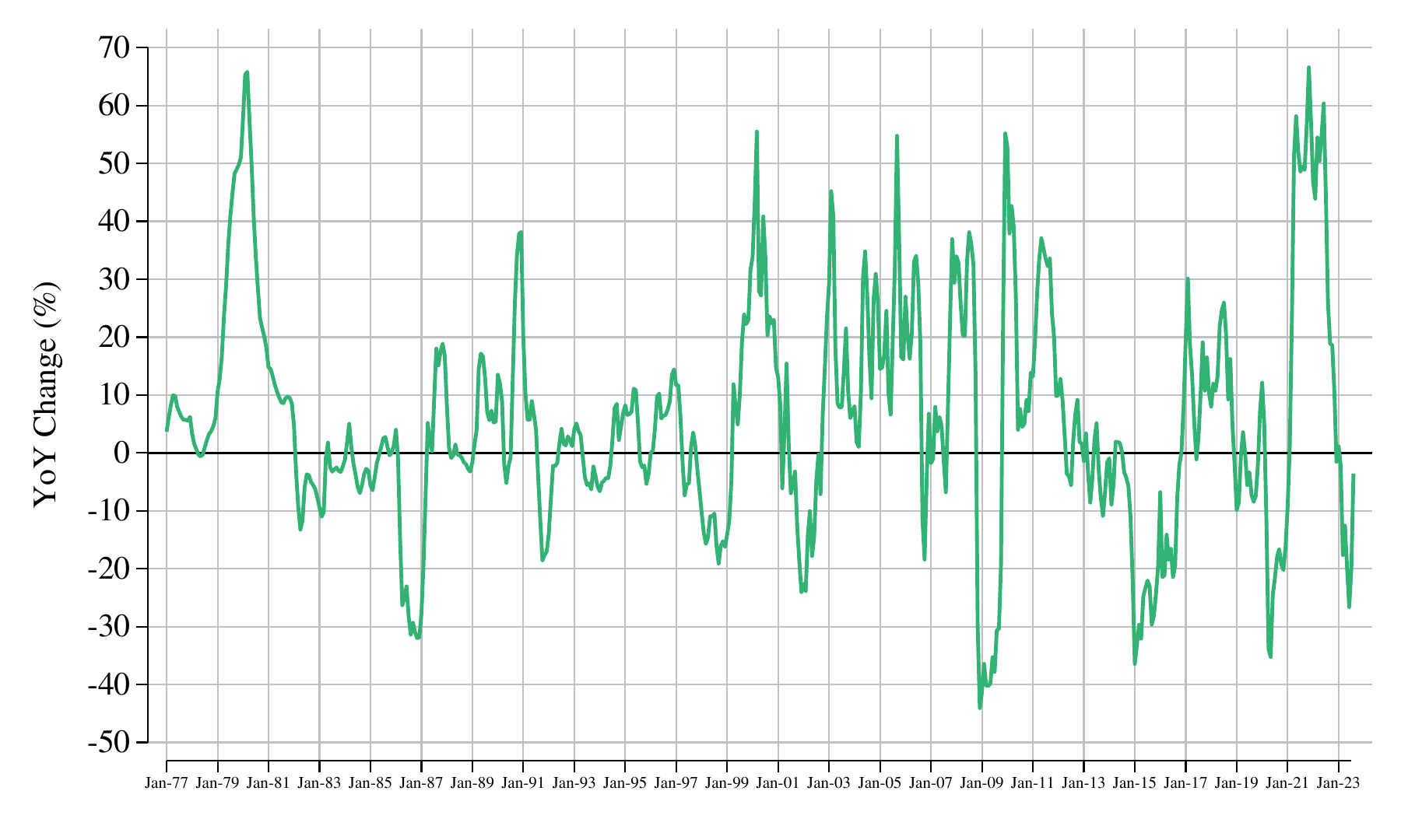
The red line in Figure [1](#fig:ie_gas_prices) shows the nominal monthly average unleaded regular gasoline price reported by the U.S. Bureau of Labor Statistics. After declining during the early stages of the COVID-19 pandemic, gasoline prices experienced an exceptional spike in 2021 and part of 2022.[^9] Nominal gasoline prices reached a record high of \$5.0 per gallon in July 2022, while annual gasoline price inflation exceeded 40% for 16 consecutive months between April 2021 and July 2022 (see Figure [A2](#fig:gas_inflation) in Appendix), the longest such spell since the 1970s.
Figure [1](#fig:ie_gas_prices) suggests a tight relation between gasoline prices and short-term IE between December 2020 and December 2022. In fact, the raw correlation between gasoline prices and median short-term IE over that period is 0.94, while the correlation of monthly and annual changes in these variables are 0.54 and 0.78, respectively. As noted by (Kilian and Zhou 2022a), however, these correlations should be interpreted with caution and could be misleading because gasoline prices may be non-stationary.
**Figure 1. Inflation Expectations and Gasoline Prices**
\
**Notes:** Median inflation expectations come from the New York Fed Survey of Consumer Expectations. Average U.S. unleaded regular gasoline prices are obtained from the U.S. Bureau of Labor Statistics. The vertical line indicates the start of Russia’s invasion of Ukraine.
Figure [1](#fig:ie_gas_prices) also shows that the empirical association between gasoline prices and medium-term IE is generally weaker. In particular, between December 2020 and December 2022, the correlation between those two variables is 0.54, while the correlation of monthly and annual changes in these variables are 0.25 and 0.20, respectively.[^10] This suggests that respondents see the influence of gasoline price changes on future inflation to decrease with the forecast horizon, consistent with the findings of (Binder 2018) or (Kilian and Zhou 2022b).
While short-term IE and gasoline price changes exhibit a strong positive covariation in 2021–2022, there are notable instances where the two series moved in opposite directions. For example, while gasoline prices dropped steeply at the start of the pandemic in early 2020, short-term IE spiked up. As gasoline prices rose sharply during the first four months of 2019 and subsequently gradually declined, IE at both horizons remained essentially flat. In early 2015, as gasoline prices rose, medium-term IE continued to trend down. Finally, between January and July 2023, gasoline prices and IE at the short- and medium-term horizons again moved in opposite directions.
## The experiment
Our objective is to evaluate the relative impact of gasoline price shocks on an individual’s short- and medium-term IE. To do so, we designed a pair of two-by-two, within-subject experiments. The four treatments in each experiment consist of asking the respondent to consider scenarios involving hypothetical price shocks to specific goods. In the first experiment, the goods are gasoline and food. In the second experiment, the goods are gasoline and durable goods. For each good, respondents are asked to consider in sequence two hypothetical price shocks of +50% and -50%. For instance, in the “negative gasoline price shock” treatment, respondents are asked: *Suppose that if instead of increasing by about 40%, the price of a gallon of gas had risen by 20% over the last 12 months.* Similarly, respondents in the “positive durable good price shock” treatment are asked: *Suppose that if instead of increasing by about 12%, the price of durable goods (such as home appliances, electronics, furniture, cars or other vehicles) had instead risen by 18% over the last 12 months.* The different treatments in each experiment and the corresponding hypothetical price change are summarized in Table [1](#tab:exper_design).[^11]
The timing of each experiment is as follows. First, respondents report their IE (point forecast) at the short-term (one-year ahead) and medium-term (three-year ahead) horizons. Then, respondents see each of the four treatments sequentially. The order of the treatments is kept fixed across respondents. The two gasoline price scenarios (positive then negative) are presented first, followed by the two price scenarios for the other good (food in experiment 1; durable goods in experiment 2).[^12] After being exposed to a given treatment, respondents are asked to report their revision in short- and medium-term IE under the corresponding scenario.
**Table 1. Experimental Design**
| | Commodity Price Inflation in Each Treatment | Commodity Price Inflation in Each Treatment | Commodity Price Inflation in Each Treatment | Commodity Price Inflation in Each Treatment |
| --- | --- | --- | --- | --- |
| | Experiment 1 | Experiment 1 | Experiment 2 | Experiment 2 |
| | Gas | Food | Gas | Durables |
| Positive Shock Treatment $= \hspace{2pt} 1.5 \hspace{2pt} \times$ Actual Annual Price Growth | 60% | 12% | 60% | 18% |
| Negative Shock Treatment $= \hspace{2pt} 0.5 \hspace{2pt} \times$ Actual Annual Price Growth | 20% | 4% | 20% | 6% |
| Number of Respondents | 1,105 | 1,105 | 1,104 | 1,104 |
**Notes**: The actual price growth rates for gas, food and durables were about 40%, 8% and 12% during the 12 months that preceded the experiment. Each cell (treatment) represents a 50% shock to these baseline rates.
We embedded these experiments in a special SCE survey fielded between May 24 and June 6, 2022. Respondents were randomly assigned to one of the two experiments and paid a fixed participation fee of \$15 upon completion of the survey. In total, 1,105 respondents participated in experiment 1, and 1,104 participated in experiment 2.
Our approach is grounded in the methodology of experimental economics. First, exposing each respondent to exogenous controlled hypothetical variations in the treatment variable should permit the causal identification of treatment effects at the individual level, thereby controlling for unobserved heterogeneity. That is, we can estimate simultaneously the causal impact of positive and negative gasoline price shocks on a respondent’s short- and medium-term IE, and this impact can be evaluated relative to other goods. Second, because the experiments were conducted within the span of two weeks, our results are mostly immune to time-varying unobserved factors and other confounds that may affect estimates based on long time-series.[^13] This is an important advantage of this experimental method: it enables identification of the causal effect of different gasoline price shocks on IE at a specific moment in time.
We acknowledge, however, that our approach may have limitations. In particular, there is no guarantee that respondents complete the survey truthfully, that they assimilate each scenario fully, that they think no other variables are changing together with the treatment variable, or that they appreciate accurately the magnitude of the shocks they are asked to consider.[^14] That said, we note that our approach belongs to a growing literature on “strategic surveys” which rely on similar hypothetical experiments to estimate parameters or associations of interest (see e.g. Armona et al. (2018), Ameriks, Briggs, Caplin, Shapiro, et al. (2020), or Andre et al. (2022)).[^15] In particular, (Armantier et al. 2022) use the same experimental design presented in this section to identify the causal effect of hypothetical inflation shocks on long-run IE. More generally, this literature has shown that the results from such hypothetical experiments are informative. As we will see next, responses in our experiment appear to be meaningful and are comparable to existing estimates.
## Sensitivity to gasoline price shocks
Results from the experiment are shown in Table [2](#tab:main_table_results). The top panel shows average normalized revisions, defined as the ratio of the individual IE revision at the one or three-year ahead horizons, and the absolute value of the hypothetical shock. This measure therefore represents the percentage point change in IE resulting from a 1.0pp change in the good’s annual price inflation. The bottom panel shows the corresponding average elasticities, defined as the ratio of the individual IE revision and the absolute value of the respondent’s IE at the corresponding horizon (one- or three-year ahead), divided by the relative size of the price shock (+50% or -50%). This second measure represents the percentage change in IE resulting from a 1% increase in the good’s annual price inflation. Following the literature (see e.g. Coibion and Gorodnichenko (2015), Binder (2018), or Kilian and Zhou (2022a)), we focus on average normalized revisions. However, with treatments all representing 50% price shocks, it also seems natural to compare elasticities.
**Table 2. Average Treatment Effect for One-Year Ahead Inflation Expectations**
| | Experiment 1 | Experiment 1 | Experiment 2 | Experiment 2 | Combined |
| --- | --- | --- | --- | --- | --- |
| | Gasoline | Food | Gasoline | Durables | Gasoline |
| | (1) | (2) | (3) | (4) | (5) |
| **Average Normalized Revisions** | **Average Normalized Revisions** | **Average Normalized Revisions** | **Average Normalized Revisions** | **Average Normalized Revisions** | **Average Normalized Revisions** |
| Positive price shock | 0.078$^{***}$ | 0.234$^{***}$ | 0.071$^{***}$ | 0.180$^{***}$ | 0.075$^{***}$ |
| | (0.004) | (0.016) | (0.003) | (0.011) | (0.002) |
| Negative price shock | -0.008$^{**}$ | -0.130$^{***}$ | -0.010$^{***}$ | -0.068$^{***}$ | -0.009$^{***}$ |
| | (0.004) | (0.018) | (0.004) | (0.012) | (0.003) |
| Observations | 1,105 | 1,105 | 1,104 | 1,104 | 2,209 |
| Positive price shock | 0.551$^{***}$ | 0.369$^{***}$ | 0.540$^{***}$ | 0.447$^{***}$ | 0.545$^{***}$ |
| | (0.033) | (0.031) | (0.029) | (0.033) | (0.022) |
| Negative price shock | 0.044 | 0.158$^{***}$ | 0.033 | 0.098$^{***}$ | 0.038$^{**}$ |
| | (0.028) | (0.025) | (0.026) | (0.027) | (0.019) |
| Observations | 1,029 | 1,029 | 1,038 | 1,038 | 2,067 |
**Notes**: Average normalized revisions are defined as the ratio of the individual inflation expectation revision and the absolute value of the corresponding commodity’s price shock. Average elasticities are defined as the ratio of the individual inflation expectation revision and the absolute value of inflation expectation divided by the relative size of the corresponding commodity’s price shock $(+50\% \hspace{3pt} \text{or} \hspace{3pt} -50\%)$. \*\*\*, \*\*, and \* indicates that the corresponding statistic is significantly different from zero at the 1%, 5% or 10% level, respectively.
We start with gasoline price shocks. The estimates in columns 1 (for experiment 1) and 3 (for experiment 2) of Table [2](#tab:main_table_results) show similarly sized effects that are not significantly different from each other (see Table [A1](#Tab:gasvgas) in Appendix). This is not surprising since respondents were randomized into experiments 1 or 2, and all saw the same gasoline price shocks in the same order. In discussing the results for gasoline price shocks, we therefore focus on the pooled sample estimates across the two experiments reported in column 5. We find that a 1.0pp increase in past-year gasoline price inflation on average leads to a significant 0.075pp upward revision in one-year ahead IE. In contrast, a 1.0pp decrease in past-year gasoline price inflation leads on average to a small but significant 0.009pp downward revision in year-ahead IE. The absolute value of this treatment effect is significantly smaller than in the +50% treatment, thereby indicating an asymmetric response of short-term IE to positive and negative gasoline price shocks. As shown in the bottom panel of Table [2](#tab:main_table_results) (column 5), these revisions translate into significant elasticities for year-ahead IE of 0.55% for positive gasoline price shocks and 0.04% for negative gasoline price shocks.
**Table 3. Average Treatment Effect for Three-Year Ahead Inflation Expectations**
| | Experiment 1 | Experiment 1 | Experiment 2 | Experiment 2 | Combined |
| --- | --- | --- | --- | --- | --- |
| | Gasoline | Food | Gasoline | Durables | Gasoline |
| | (1) | (2) | (3) | (4) | (5) |
| **Average Normalized Revisions** | **Average Normalized Revisions** | **Average Normalized Revisions** | **Average Normalized Revisions** | **Average Normalized Revisions** | **Average Normalized Revisions** |
| Positive price shock | 0.054$^{***}$ | 0.203$^{***}$ | 0.047$^{***}$ | 0.149$^{***}$ | 0.051$^{***}$ |
| | (0.004) | (0.016) | (0.004) | (0.011) | (0.003) |
| Negative price shock | 0.002 | -0.061$^{***}$ | -0.004 | -0.045$^{***}$ | -0.001 |
| | (0.003) | (0.016) | (0.004) | (0.012) | (0.002) |
| Observations | 1,105 | 1,105 | 1,104 | 1,104 | 2,209 |
| Positive price shock | 0.434$^{***}$ | 0.404$^{***}$ | 0.470$^{***}$ | 0.429$^{***}$ | 0.452$^{***}$ |
| | (0.048) | (0.043) | (0.040) | (0.035) | (0.031) |
| Negative price shock | -0.028 | 0.087$^{***}$ | 0.007 | 0.064$^{**}$ | -0.010 |
| | (0.033) | (0.025) | (0.029) | (0.026) | (0.022) |
| Observations | 1,028 | 1,028 | 1,045 | 1,045 | 2,073 |
**Notes**: Average normalized revisions are defined as the ratio of the individual inflation expectation revision and the absolute value of the corresponding commodity’s price shock. Average elasticities are defined as the ratio of the individual inflation expectation revision and the absolute value of inflation expectation divided by the relative size of the corresponding commodity’s price shock $(+50\% \hspace{3pt} \text{or} \hspace{3pt} -50\%)$. \*\*\*, \*\*, and \* indicates that the corresponding statistic is significantly different from zero at the 1%, 5% or 10% level, respectively.
The results in column 5 of Table [3](#tab:main_table_results_3yr) show a significant (insignificant) average normalized revision of 0.051pp (-0.001pp) in three-year ahead IE in response to a 1.0pp increase (decrease) in past-year gasoline price inflation. The corresponding elasticities are 0.45% for positive and -0.01% for negative gasoline price shocks. Two points are worth noting in Table [3](#tab:main_table_results_3yr). First, the treatment effects are significantly smaller for three- than for one-year ahead IE. Hence, respondents expect the impact of gasoline price shocks on IE to fade with the forecast horizon, consistent with e.g. (Binder 2018) or (Kilian and Zhou 2022b). Second, the average absolute revision in three-year ahead IE is significantly smaller for negative than for positive gasoline price shocks. Thus, we find the same asymmetry in the effect of positive and negative gasoline price shocks on one- and three-year ahead IE revisions.
## Heterogeneity in the sensitivity to gasoline price shocks
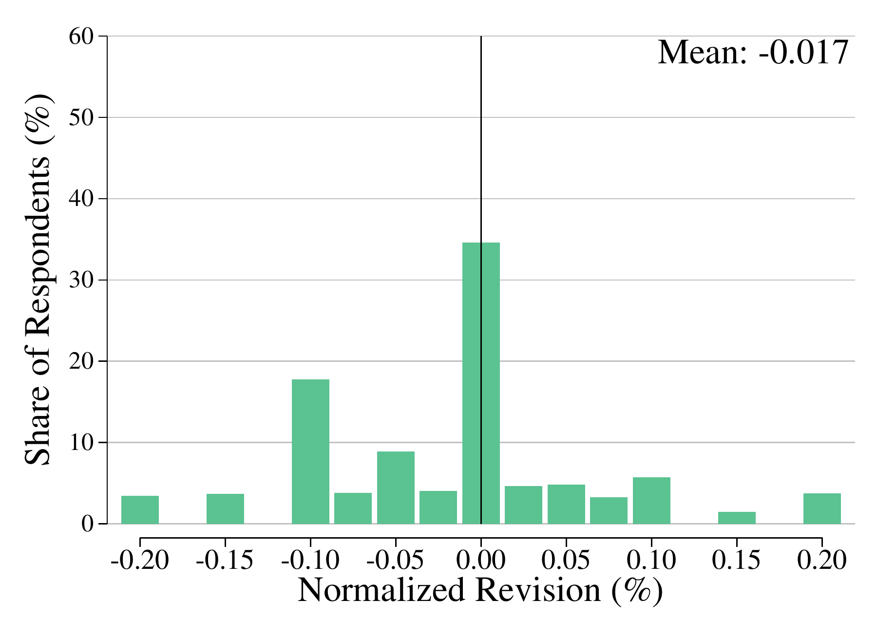
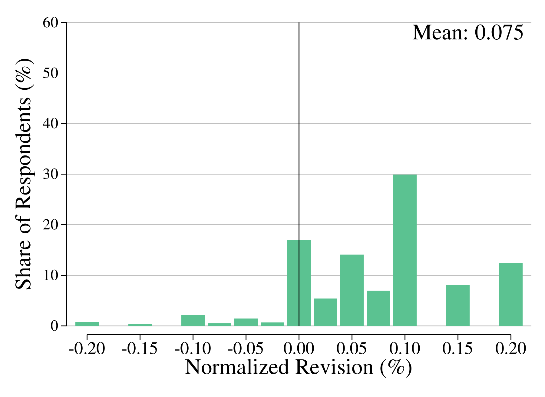
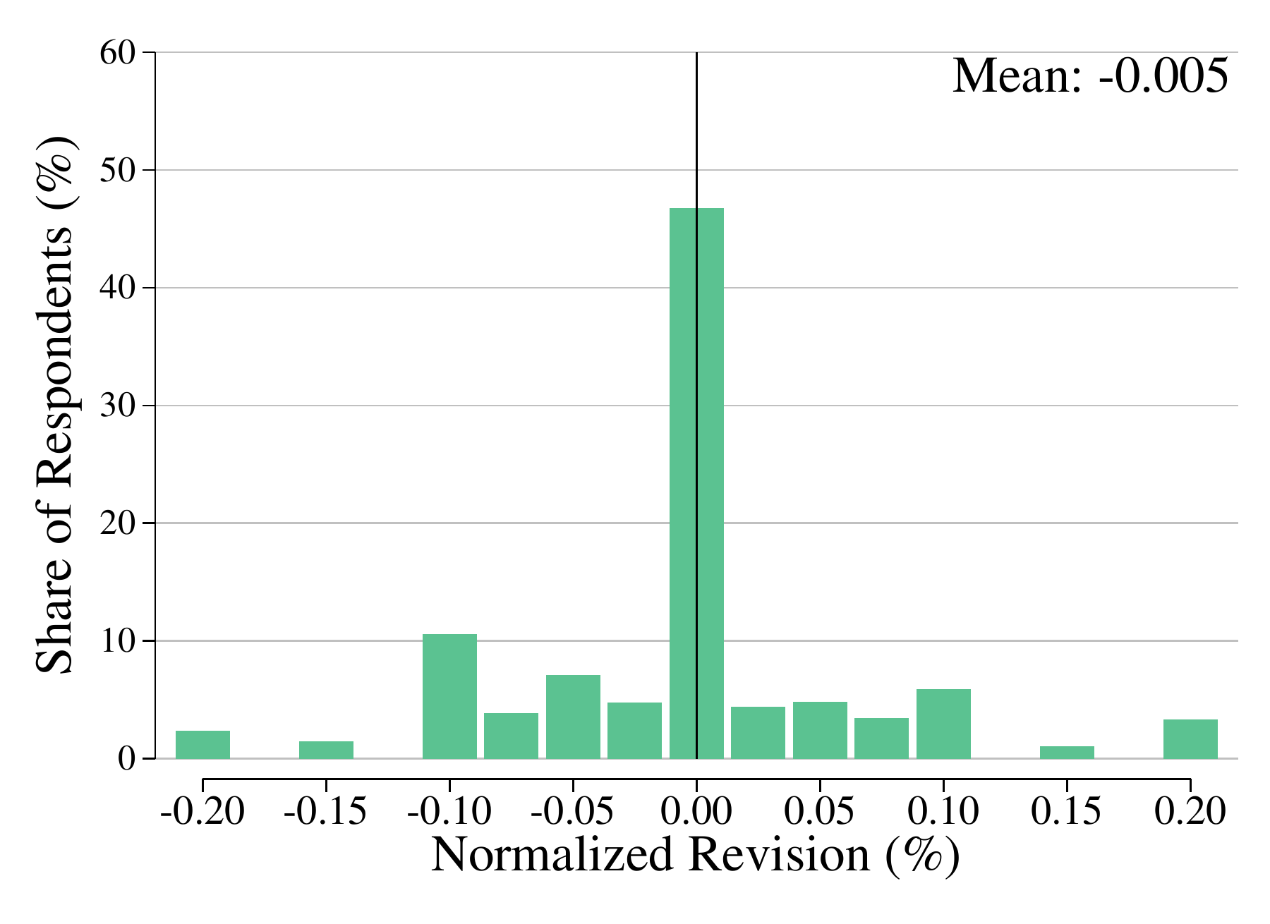
To explore possible heterogeneity in responses across respondents, we plot in Figure [2](#fig:side_by_side_gas) the distribution of individual normalized revisions. The figure shows considerable heterogeneity across respondents in their perceived sensitivity of IE to gasoline price shocks. Interestingly, about 17% percent of respondents report no contribution of positive past-year gasoline price shocks on their short-term IE, while about 35% report no contribution from gasoline price declines.[^16] The proportion of respondents reporting zero responsiveness in their medium-term IE is even higher (almost 33% for positive and 47% for negative shocks). Further, when faced with a positive (negative) shock, only 19% (33%) of respondents revised their three-year ahead IE upward (downward) more than their year-ahead IE. These results support the hypothesis that most respondents see the effect of gasoline price shocks on future inflation as transitory.
**Figure 2. Distribution of Normalized Revisions**
**One-Year Ahead Inflation Expectations (%)**
**Negative Gasoline Price Shock**
**Positive Gasoline Price Shock**
**Three-Year Ahead Inflation Expectations (%)**
**Negative Gasoline Price Shock**
**Positive Gasoline Price Shock**
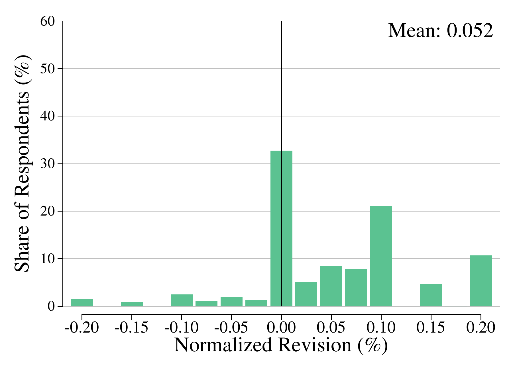
Figure [2](#fig:side_by_side_gas) also shows that the distribution of normalized revisions has more mass away from zero in the positive than in the negative shock treatments. This result reflects the fact that most respondents (80% at the one- and 82% at the three-year ahead horizon) report absolute revisions in the positive shock treatment that are greater than or equal to their absolute revisions in the negative shock treatment. These results therefore provide clear support to the hypothesis that most respondents update their IE asymmetrically when faced with a positive or a negative gasoline price shock.
**Table 4. Heterogeneity Analysis: Normalized Revisions**
| | Normalized Revisions in One-Year Ahead IE | Normalized Revisions in One-Year Ahead IE | Normalized Revisions in Three-Year Ahead IE | Normalized Revisions in Three-Year Ahead IE |
| --- | --- | --- | --- | --- |
| | (1) | (2) | (3) | (4) |
| | Negative Gasoline Price Shock | Positive Gasoline Price Shock | Negative Gasoline Price Shock | Positive Gasoline Price Shock |
| Female | 0.015$^{***}$ | 0.001 | 0.014$^{***}$ | 0.004 |
| | (0.006) | (0.005) | (0.005) | (0.006) |
| Non-White | -0.000 | -0.015$^{*}$ | -0.002 | -0.006 |
| | (0.008) | (0.008) | (0.008) | (0.009) |
| Married | -0.007 | 0.000 | -0.010$^{*}$ | -0.004 |
| | (0.006) | (0.006) | (0.006) | (0.006) |
| High School or Less | 0.006 | -0.001 | -0.002 | 0.001 |
| | (0.008) | (0.007) | (0.007) | (0.008) |
| College Graduate | -0.015$^{***}$ | -0.007 | -0.008$^{*}$ | 0.004 |
| | (0.005) | (0.005) | (0.005) | (0.005) |
| 36 $\leq$ Age $<$ 55 | -0.000 | -0.003 | 0.002 | -0.001 |
| | (0.007) | (0.006) | (0.007) | (0.008) |
| Age $\geq$ 55 | -0.016$^{**}$ | -0.014$^{**}$ | -0.016$^{**}$ | -0.006 |
| | (0.007) | (0.006) | (0.006) | (0.008) |
| Household Income $\leq$50K | -0.002 | 0.003 | -0.005 | 0.010 |
| | (0.006) | (0.006) | (0.006) | (0.007) |
| Household Income $>$ 100k | 0.010 | 0.004 | 0.005 | 0.011$^{*}$ |
| | (0.007) | (0.006) | (0.006) | (0.006) |
| High Numeracy | -0.014$^{**}$ | 0.011$^{*}$ | -0.009 | 0.004 |
| | (0.007) | (0.006) | (0.006) | (0.007) |
| Risk Tolerance | 0.002 | -0.003$^{**}$ | -0.000 | -0.004$^{**}$ |
| | (0.002) | (0.002) | (0.002) | (0.002) |
| Constant | -0.001 | 0.088$^{***}$ | 0.016 | 0.058$^{***}$ |
| | (0.014) | (0.012) | (0.012) | (0.013) |
| Adj. R-Squared | 0.034 | 0.013 | 0.026 | 0.007 |
| Dep. Var Mean | -0.009 | 0.075 | -0.001 | 0.051 |
| Observations | 2,186 | 2,186 | 2,186 | 2,186 |
**Note**: Results of linear regressions in which the dependent variable is the individual normalized revisions in one- and three-year ahead inflation expectations in response to +50% and -50% gasoline price inflation shocks. To measure risk tolerance respondents are asked to report their willingness to take risks regarding financial matters using a Likert scale ranging from 1 (not willing at all) to 7 (very willing). A respondent is classified as having high numeracy when they answers correctly at least four out of five numeracy and financial literacy questions based on (Lusardi and Mitchell 2007).
To test for possible differences between demographic groups, we regress individual normalized revisions in each treatment on demographic characteristics (see Table [4](#table:gasheterogeneity)).[^17] The estimated constant terms in columns 2 and 4 (1 and 3) confirm the significant (insignificant) effect of positive (negative) gasoline price shocks on individual IE. Further, the treatment effects appear fairly broad-based as few of the demographic characteristics are significant. Specifically, older and college-educated respondents revise their IE downward more in response to a negative gasoline price shock. Conversely, women seem less responsive to negative gasoline price shocks. Finally, respondents with higher financial literacy and numeracy tend to be more responsive to gasoline shocks.
We also explore the extent to which there is heterogeneity in how participants update their IE asymmetrically in response to positive and negative gasoline price shocks. To do so, we run a regression in which the dependent variable is a measure of individual asymmetry at a given horizon, defined as the difference between a respondent’s absolute normalized revision in the positive price shock treatment and her absolute normalized revision in the negative price shock treatment.
The estimated constant terms in Table [5](#table:Asymheterogeneity) confirm the presence of a significant asymmetry at both horizons, with stronger IE revisions in response to positive than negative gasoline price shocks. The asymmetry appears to be broad-based as most demographic characteristics are not significantly different from zero. Nevertheless, we find that college graduates exhibit slightly more asymmetry in their three-year ahead IE revisions. In contrast, older respondents are significantly more symmetric in the way they respond to positive and negative gasoline price shocks. This result is interesting as it confirms the important role age plays in consumers’ IE formation and updating. Since the influential contribution of (Malmendier and Nagel 2016), it has been well established that older respondents tend to have higher IE (see also Armantier et al. (2021)).[^18] (Malmendier and Nagel 2016) argue that this finding reflects the fact that older respondents are more likely to have experienced high inflation periods in their lifetime (e.g. in the 1970s). The results in this section add to the literature by showing that older respondents revise their IE downward more in response to negative gasoline price shocks and that their updating process is more symmetric when faced with positive and negative price fluctuations. Consistent with (Malmendier and Nagel 2016)’s hypothesis, these results may be due to the fact that older people are more likely to have experienced substantial positive and negative gasoline price shocks during their lifetime.[^19]
**Table 5. Heterogeneity Analysis: Asymmetric Responses**
| | \(1\) | \(2\) |
| --- | --- | --- |
| | One-Year Ahead | Three-Year Ahead |
| Female | -0.098 | -0.028 |
| | (0.093) | (0.097) |
| Non-White | -0.067 | -0.123 |
| | (0.131) | (0.121) |
| Married | 0.107 | 0.166 |
| | (0.110) | (0.115) |
| High School or Less | 0.045 | 0.137 |
| | (0.136) | (0.136) |
| College Graduate | 0.039 | 0.149$^{*}$ |
| | (0.091) | (0.089) |
| 36 $\leq$ Age $<$ 55 | -0.107 | -0.177 |
| | (0.133) | (0.125) |
| Age $\geq$ 55 | -0.520$^{***}$ | -0.296$^{**}$ |
| | (0.138) | (0.132) |
| Household Income $\leq$50K | 0.030 | -0.067 |
| | (0.117) | (0.131) |
| Household Income $>$ 100k | -0.040 | -0.108 |
| | (0.098) | (0.094) |
| High Numeracy | 0.120 | 0.082 |
| | (0.118) | (0.119) |
| Risk Tolerance | -0.040 | -0.050$^{*}$ |
| | (0.028) | (0.029) |
| Constant | 0.800$^{***}$ | 0.659$^{***}$ |
| | (0.225) | (0.206) |
| Adj. R-Squared | 0.021 | 0.012 |
| Dep. Var Mean | 0.516 | 0.472 |
| Observations | 2,186 | 2,186 |
\
## Sensitivity to food and durable good price shocks
How does the effect of gasoline prices on IE compare to the effect of other goods? The top panel of Table [2](#tab:main_table_results) (columns 2 and 4) shows that revisions in year-ahead IE in response to a 1.0pp increase in food and durable good prices are 0.234pp and 0.180pp, respectively. Hence, the impact of an increase in food or in durable good price inflation on short-term IE is 3.1 and 2.4 times larger than the impact of an identical increase in gasoline price inflation (these differences are significant at the 1% level). In contrast, positive price shock elasticities of year-ahead IE for food and durable goods (0.37% and 0.45% in columns 2 and 4 in the bottom panel of Table [2](#tab:main_table_results)) are smaller than for gasoline prices. The difference, however, is only significant for food prices. Table [2](#tab:main_table_results) shows that short-term IE revisions are again asymmetric, with significantly (at the 1% level) lower sensitivity of IE to negative food and durable good price shocks than to positive price shocks.
Table [3](#tab:main_table_results_3yr) shows that revisions in three-year ahead IE in response to food and durable good price shocks display similar but weaker patterns than revisions in year-ahead IE. The normalized revisions for positive food and durable good price shocks are respectively 4.0 and 2.9 times larger than that for gasoline price increases (these differences are significant at the 1% level). While more responsive than for gasoline price shocks, normalized revisions to negative food and durable good price shocks remain considerably (and significantly at the 1% level) smaller than those for positive food and durable good price growth shocks. Finally, elasticities of three-year ahead IE to food and durable good price inflation increases (decreases) are 0.40% and 0.43% (0.09% and 0.06%) in the bottom panel of Table [3](#tab:main_table_results_3yr).
(Binder 2018) argues that a natural benchmark to compare normalized IE revisions in response to price shocks across different goods is their relative importance in household spending baskets. When our experiment was conducted, the relative importance of food, durable goods, and gasoline in the CPI was 13.5%, 12.6% and 3.3%, respectively. Based solely on these relative weights, one could have expected normalized revisions in IE to food and durable good price increases to be approximately 4.1 and 3.8 times larger than those for gasoline prices. As shown in Table [6](#tab:ratio_summary), this is slightly higher (much lower) than the normalized revisions ratios we found in the positive (negative) price shock treatment.
\[h\]
**Table 6. Expected and Actual Year-Ahead Normalized Revision Ratios**
| | Food to Gasoline | Durables to Gasoline |
| --- | --- | --- |
| Expected ratio based only on CPI weights | 4.1 | 3.8 |
| Expected ratio including indirect effects | 3.4 | 3.2 |
| Actual ratio in positive shock treatment | 3.1 | 2.4 |
| Actual ratio in negative shock treatment | 14.4 | 7.6 |
**Note**: Expected ratios based on CPI weights are defined as the good’s CPI weight divided by gasoline’s CPI weight. Expected ratios based on indirect effects use an adjusted CPI weight for gasoline that takes into account its indirect effects as per (Kilian and Zhou 2023a). Actual ratio is the average normalized revision for the good divided by the average normalized revision for gasoline.
When considering the full impact of gasoline price changes on IE, however, respondents should include the indirect effect of gasoline price changes on the prices of other goods. (Kilian and Zhou 2023a) find the response of (realized) inflation to a 1.0pp nominal gasoline price shock to be 0.04pp. Using this measure of relative importance, one would then expect normalized revisions in IE to food and durable good price increases to be approximately 3.4 and 3.2 times larger than those for gasoline prices. As can be seen in Table [6](#tab:ratio_summary), these ratios are closer to (further away from) the ones we obtained in the positive (negative) shock treatment.[^20]
Summing up, consistent with (Binder 2018), we find no evidence suggesting that gasoline prices have an outsized effect on IE. In particular, the sensitivity of IE to positive (negative) gasoline price shocks appears to be consistent (low) relative to the expenditure share of gasoline in households’ spending basket.[^21]
## Counterfactual simulation exercise
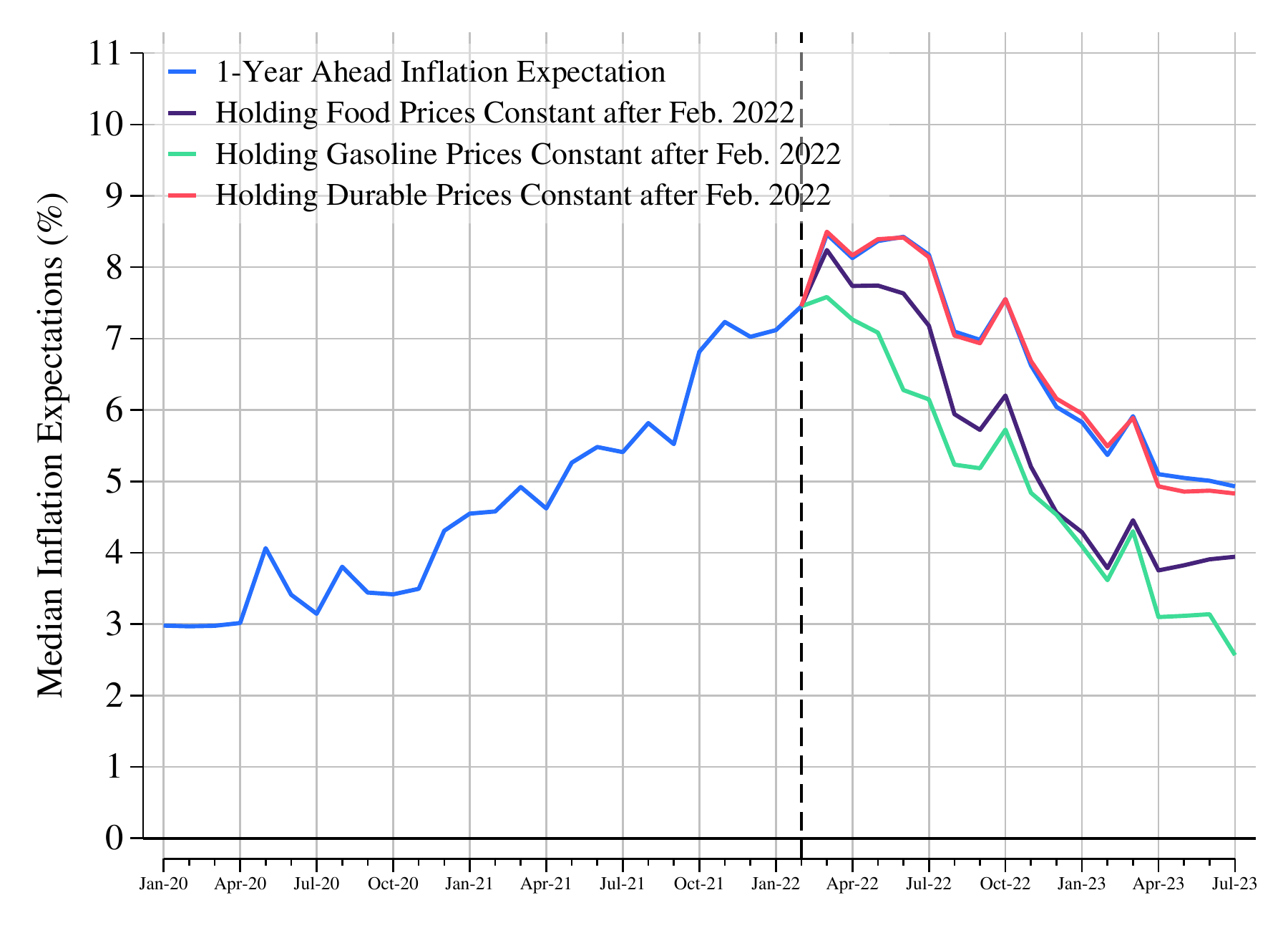
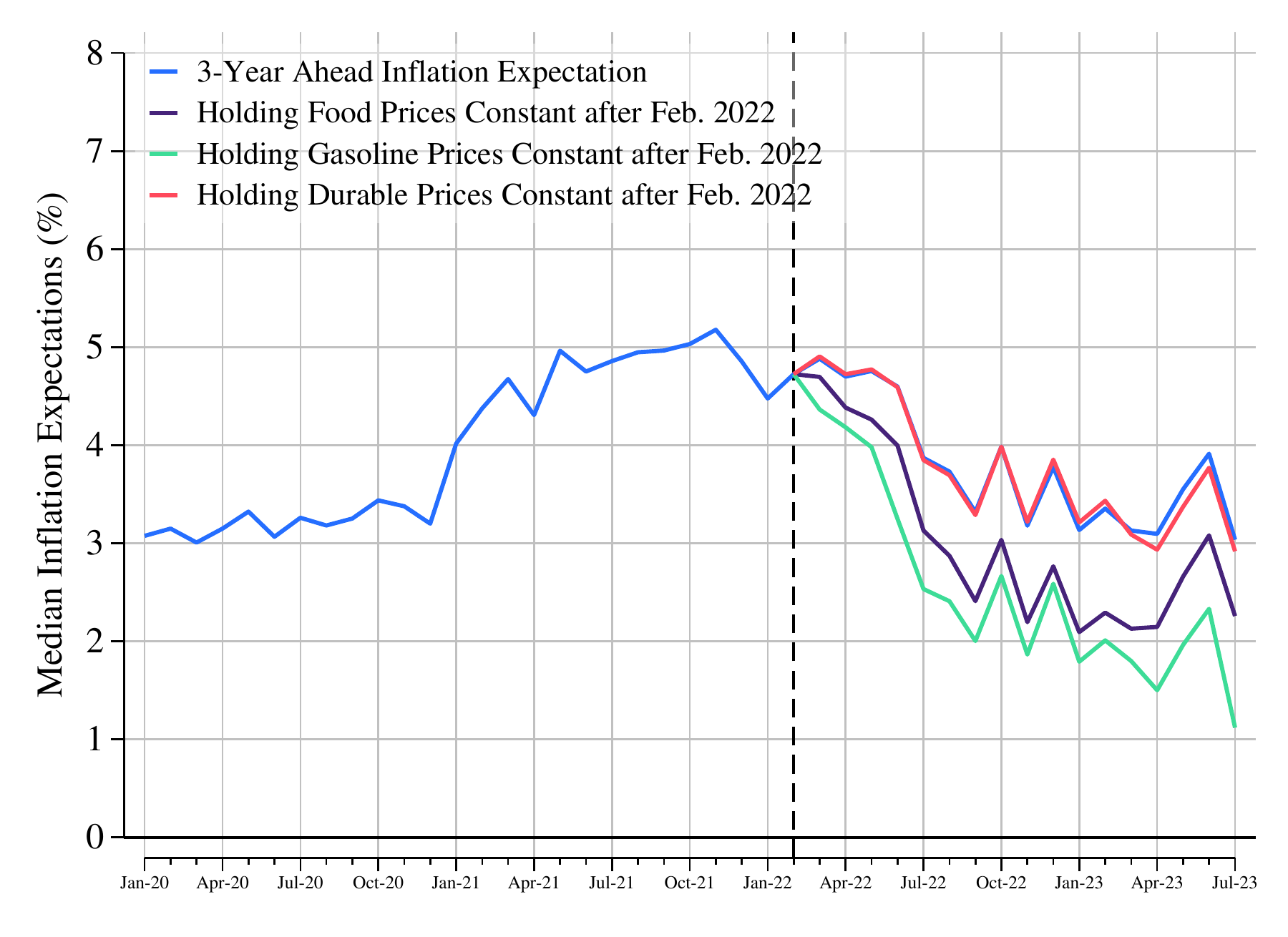
(Binder 2018) argues that because gasoline prices often experience large fluctuations, their contribution to IE may be substantial even if the sensitivity of IE to gasoline price changes is relatively small. To illustrate this point, we conduct a counterfactual exercise in which we study the post-Ukraine-invasion evolution of IE when i) gasoline price levels are fixed at their February 2022 values, and ii) the sensitivity of IE to gasoline prices is set at the level estimated in Section 4.1.[^22] Specifically, we recursively deduct each month’s gasoline-price-change contribution to IE, starting on March 1, 2022 and moving forward using the estimates in Tables [2](#tab:main_table_results) and [3](#tab:main_table_results_3yr) corresponding to positive and negative gasoline price shocks.[^23]
**Figure 3. Counterfactual Exercises for Different Commodities**
**One-Year Ahead Inflation Expectations (%)**
**Three-Year Ahead Inflation Expectations (%)**
**Note**: Median inflation expectations come from the New York Fed Survey of Consumer Expectations. The vertical line indicates the start of Russia’s invasion of Ukraine. See Appendix B for detail on the implementation of the counterfactual exercise.
Comparing the blue (actual) and green (counterfactual) IE series in the left panel of Figure [3](#fig:counterfactual1) suggests that, all else equal, one-year ahead IE would have risen substantially less post-invasion under the counterfactual. Further, IE would have fallen below 5.0% by November 2022, instead of by July 2023. Similarly, the right panel of Figure [3](#fig:counterfactual1) shows that the three-year ahead IE would have fallen below 3.1% by July 2022, instead of by July 2023.
To gauge the relative magnitude of these effects, we conduct the same counterfactual exercise with food and durable good prices. The food prices simulation (purple line in Figure [3](#fig:counterfactual1)) shows a relatively similar (albeit somewhat weaker) influence as the gasoline prices simulation on the post-invasion evolution of IE at both horizons. In contrast, durable goods (red line in Figure [3](#fig:counterfactual1)) would have had essentially no impact on the dynamics of IE during the same period. This counterfactual exercise suggests that while post-invasion increases in gasoline and food price inflation may have helped prolong high IE levels during 2022, durable good prices instead played a minor role.
**Figure 4. Gasoline Counterfactual Exercises for Different Time Periods**
**One-Year Ahead Inflation Expectations (%)**
**Three-Year Ahead Inflation Expectations (%)**
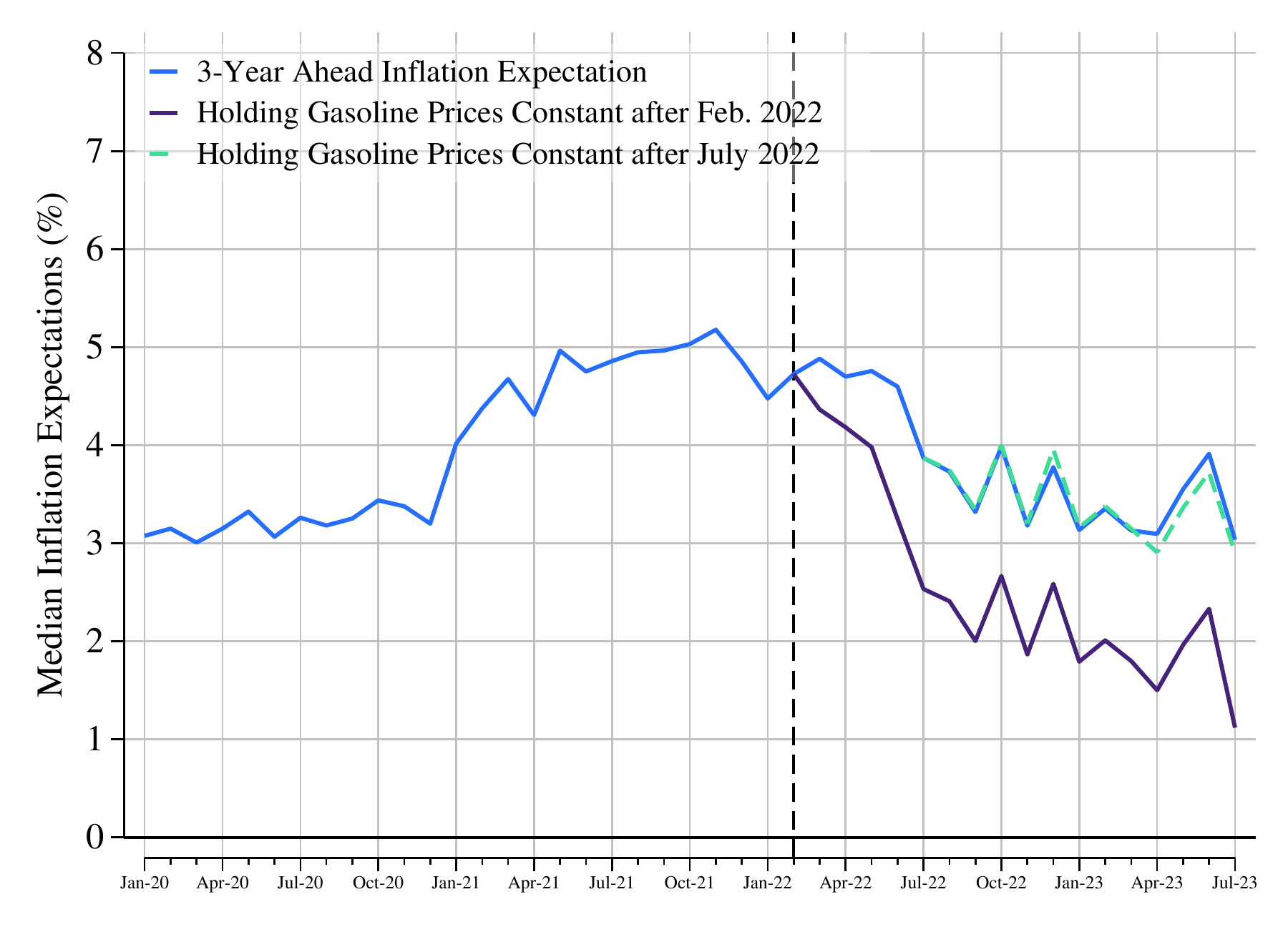
**Notes**: Median inflation expectations come from the New York Fed Survey of Consumer Expectations. The vertical line indicates the start of Russia’s invasion of Ukraine. See Appendix B for detail on the implementation of the counterfactual exercise.
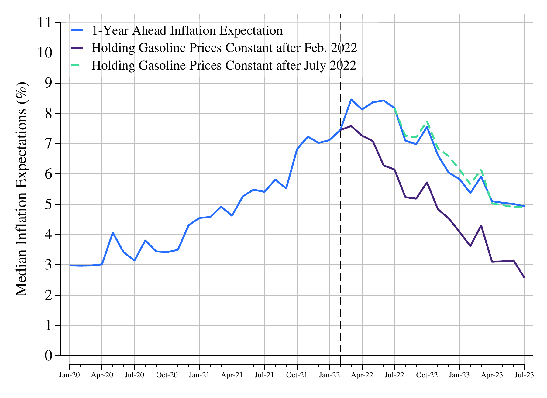
Observe that most of the gasoline price effects in Figure [3](#fig:counterfactual1) are concentrated around the few months that followed the Russian invasion of Ukraine. After that, the difference between actual IE and simulated IE remains relatively constant. This result may be due in part to the fact that gasoline prices reached their peak in July 2023, after which they started declining (see Figure [1](#fig:ie_gas_prices)). The relatively low responsiveness of IE to negative gasoline price changes we identified in our experiment could then explain the small difference between actual and simulated IE in Figure [3](#fig:counterfactual1) after July 2022. To explore this possibility, we conducted the same counterfactual experiment except that gasoline price levels are now fixed at their July (instead of February) 2022 values. The results in Figure [4](#fig:counterfactual2) show little difference between the simulated trajectory of IE (dotted green line) and actual IE (blue line). Hence, while the sharp increase in gasoline prices that followed the Russian invasion of Ukraine seems to have had a substantial impact on consumers’ IE, the subsequent decrease in gasoline prices that started in July 2022 was mostly innocuous. The latter result is consistent with (Kilian and Zhou 2023a) who find no evidence that gasoline price shocks had a notable effect on IE between June 2022 and December 2023.
## Discussion
This paper reports on an experiment that shows that IE respond to hypothetical gasoline price shocks during a period of high gasoline and headline inflation. The results also indicate that the sensitivity of IE to gasoline price shocks declines with the forecast horizon and is asymmetric, whereby positive shocks have a significantly greater impact than negative shocks. Namely, one- and three-year ahead IE increase on average by 0.075pp and 0.051pp in response to a positive 1.0pp gasoline price increase and decline on average by 0.009pp and 0.001pp in response to a 1.0pp gasoline price decrease. These estimated contributions of gasoline price are relatively small when compared to the contributions of food and durable good price shocks to IE (3.1 and 2.4 smaller, respectively). Further, we find no evidence suggesting that gasoline prices have an outsized effect on IE. In fact, the sensitivity of IE to negative gasoline price shocks is disproportionately low relative to the expenditure share of gasoline in households’ basket. Consistent with these results, a counterfactual exercise shows that the sharp Ukraine-invasion-induced increase in gasoline prices had a substantial impact on IE dynamics in the first half of 2022, whereas the post-July 2022 decrease in gasoline prices was mostly inconsequential.
How do our experimental estimates compare to those obtained with times-series data? (Binder 2018) estimates that a 1.0pp increase in gasoline prices results in a 0.01pp increase in year-ahead IE, as reported in the Michigan Survey of Consumers. Although measured somewhat differently, (Kilian and Zhou 2022b) find that a gasoline price shock of 1.0pp raises IE by 0.03pp. These estimates, however, do not distinguish between positive and negative gasoline price shocks. Therefore, they are not directly comparable to ours. When we combine our results for the +50% and -50% treatments, we find that a 1.0pp change in gasoline prices leads to an overall change of 0.03pp in year-ahead IE on average. Therefore, our experiment produced causal estimates of the contribution to year-ahead IE which are comparable to those recently in recent studies.
Our experimental study adds to the existing literature in several ways. First, contrary to widespread and persistent beliefs, but consistent with recent literature (e.g. Binder (2018) or Kilian and Zhou (2022a)), we find new causal evidence that the sensitivity of IE to gasoline price shocks is not disproportionate. Contrary to the statements reported in the introduction, this suggests that movements in short-term IE should not be attributed to gasoline price changes alone. Further, the modest response to negative gasoline price shocks in our experiment suggests that one may essentially ignore decreases in gasoline prices when considering the impact on IE.
Second, the clear asymmetry in IE responses to positive and negative price shocks we identify is new and surprising. In particular, finding that older respondents tend to update their IE more symmetrically than their peers supports (Malmendier and Nagel 2016)’s hypothesis that personal inflation experience plays a major role in shaping individual IE. Further, our results echo the long literature suggesting that changes in money supply can have asymmetric effects (e.g. Ball and Romer (1990) or Cover (1992)). In particular, the experiments of (Fehr and Tyran 2001), (Noussair et al. 2012) and (Duffy and Puzzello 2014) show that prices respond less to deflationary than to inflationary shocks. Our results show similar asymmetric responses of IE to price shocks. Going forward, it may be interesting to explore the extent to which expectations play a role in explaining the non-neutrality of money.
Third, we find the impact of the three goods’ price shocks on future inflation to be somewhat persistent. For example, we find that a 1.0pp change in gasoline prices leads to a 0.025pp change in the same direction in three-year ahead IE. While smaller than the effects on short-term expectations, our estimates imply some perceived persistence in the effect of gasoline price changes on medium-term inflation. Policymakers are concerned about factors that may contribute to an un-anchoring of long-term IE. Our study cannot speak directly to this issue since we focused on the short- and medium-term horizons. Nevertheless, following (Kilian and Zhou 2023b), it will be important to extend our work to assess the extent to which our persistence result extend to longer-term expectations. Nevertheless, it will be important to extend our work to confirm the results of (Kilian and Zhou 2023b) which suggest that the effect of gasoline price shocks do not extend to long-term IE.
Our paper raises several interesting questions that could be addressed in future research. In particular, building on (Aastveit et al. 2023) who find that households’ IE respond more to demand-driven crude oil price shocks than supply shocks, one might explore whether the IE sensitivity we find in the experiment depends on the factors that cause a gasoline price shock. Further, it would be interesting to test the extent to which consumers’ IE respond differently to endogenous gasoline price shocks (e.g. due to demand shifts) or to exogenous shocks (e.g. due to local productivity shocks as in Andre et al. (2022)). Replicating our experiment at different time periods (e.g. when gasoline prices are low and stable) should also shed light on the extent to which the sensitivity and the asymmetry of consumers’ IE revisions in response to gasoline price shocks vary over time. Finally, one should study whether there are non-linearities in the way households revise their IE in response to gasoline price shocks of different sizes. Are consumers relatively more or less sensitive to larger shocks? Our experimental design could be easily modified to address these issues by specifying different shock sizes or different narratives.
To conclude, we would like to stress the importance of finding similar sensitivity estimates in our experiment as those obtained in the recent applied econometric literature with times series (field) data. As a proof of concept, it is an encouraging result which supports the use of experiments to study questions related to macroeconomic and monetary policy. Going forward, the advantages of the experimental approach we have exploited in this paper should prove useful in shedding new light on other issues that have been long-standing in the monetary policy literature.
## Appendix A. Additional Figures and Tables
**Table A1. Two-sample T-Statistics for Difference across Experiments in Average Normalized Revision to Gas Price Shocks**
| | One-Year Ahead | Three-Years Ahead |
| --- | --- | --- |
| Test-Statistic for Difference in Average Normalized Revisions | Test-Statistic for Difference in Average Normalized Revisions | Test-Statistic for Difference in Average Normalized Revisions |
| Positive price shock treatment | 1.4 | 1.2 |
| Negative price shock treatment | 0.4 | 1.2 |
| Positive price shock treatment | 0.3 | -0.6 |
| Negative price shock treatment | 0.3 | -0.8 |
| Observations | 2,209 | 2,209 |
**Table A2. Average Normalized Revision for One-Year Ahead Inflation Expectations by Demographic Group**
| | Gasoline Price Treatment | Gasoline Price Treatment |
| --- | --- | --- |
| | (1) | (2) |
| | Lower | Higher |
| Overall | -0.009$^{***}$ | 0.075$^{***}$ |
| Female | 0.000 | 0.076$^{***}$ |
| Male | -0.020$^{***}$ | 0.074$^{***}$ |
| White | -0.011$^{***}$ | 0.078$^{***}$ |
| Non-White | -0.001 | 0.062$^{***}$ |
| Married | -0.013$^{***}$ | 0.076$^{***}$ |
| High School or Less | -0.001 | 0.074$^{***}$ |
| Some College | -0.006 | 0.077$^{***}$ |
| College Graduate | -0.020$^{***}$ | 0.073$^{***}$ |
| Age $\leq$ 35 | -0.005 | 0.079$^{***}$ |
| 36 $\leq$ Age $<$ 55 | -0.001 | 0.077$^{***}$ |
| Age $\geq$ 55 | -0.018$^{***}$ | 0.071$^{***}$ |
| Household Income $\leq$50K | -0.005 | 0.075$^{***}$ |
| 50K $<$ Household Income $\leq$100K | -0.014$^{***}$ | 0.073$^{***}$ |
| Household Income $>$ 100k | -0.010$^{**}$ | 0.076$^{***}$ |
| High Numeracy | -0.017$^{***}$ | 0.078$^{***}$ |
| Low Numeracy | 0.005 | 0.069$^{***}$ |
**Notes**: Table reports average normalized revisions for one-year ahead inflation expectations in response to +50% and -50% gasoline price inflation shocks by demographic group. Average normalized revisions are defined as the ratio of the individual inflation expectation revision and the absolute value of the price shock. \*\*\*, \*\*, and \* indicates that the corresponding statistic is significantly different from zero at the 1%, 5% or 10% level, respectively. A respondent is classified as having high numeracy when they answer correctly at least four out of five numeracy and financial literacy questions based on (Lusardi and Mitchell 2007).
**Table A3. Average Normalized Revision for Three-Year Ahead Inflation Expectations by Demographic Group**
| | Gasoline Price Treatment | Gasoline Price Treatment |
| --- | --- | --- |
| | (1) | (2) |
| | Lower | Higher |
| Overall | -0.001 | 0.051$^{***}$ |
| Female | 0.008$^{*}$ | 0.054$^{***}$ |
| Male | -0.010$^{***}$ | 0.047$^{***}$ |
| White | -0.002 | 0.052$^{***}$ |
| Non-White | 0.004 | 0.046$^{***}$ |
| Married | -0.005$^{*}$ | 0.049$^{***}$ |
| High School or Less | 0.001 | 0.051$^{***}$ |
| Some College | 0.002 | 0.049$^{***}$ |
| College Graduate | -0.005$^{***}$ | 0.053$^{***}$ |
| Age $\leq$ 35 | 0.004 | 0.052$^{***}$ |
| 36 $\leq$ Age $<$ 55 | 0.007$^{*}$ | 0.052$^{***}$ |
| Age $\geq$ 55 | -0.010$^{**}$ | 0.049$^{***}$ |
| Household Income $\leq$50K | 0.001 | 0.055$^{***}$ |
| 50K $<$ Household Income $\leq$100K | -0.003 | 0.044$^{***}$ |
| Household Income $>$ 100k | -0.001 | 0.054$^{***}$ |
| High Numeracy | -0.006$^{**}$ | 0.051$^{***}$ |
| Low Numeracy | 0.008 | 0.050$^{***}$ |
**Notes**: Table reports average normalized revisions for three-year ahead inflation expectations in response to +50% and -50% gasoline price inflation shocks by demographic group. Average normalized revisions are defined as the ratio of the individual inflation expectation revision and the absolute value of the price shock. \*\*\*, \*\*, and \* indicates that the corresponding statistic is significantly different from zero at the 1%, 5% or 10% level, respectively. A respondent is classified as having high numeracy when they answer correctly at least four out of five numeracy and financial literacy questions based on (Lusardi and Mitchell 2007).
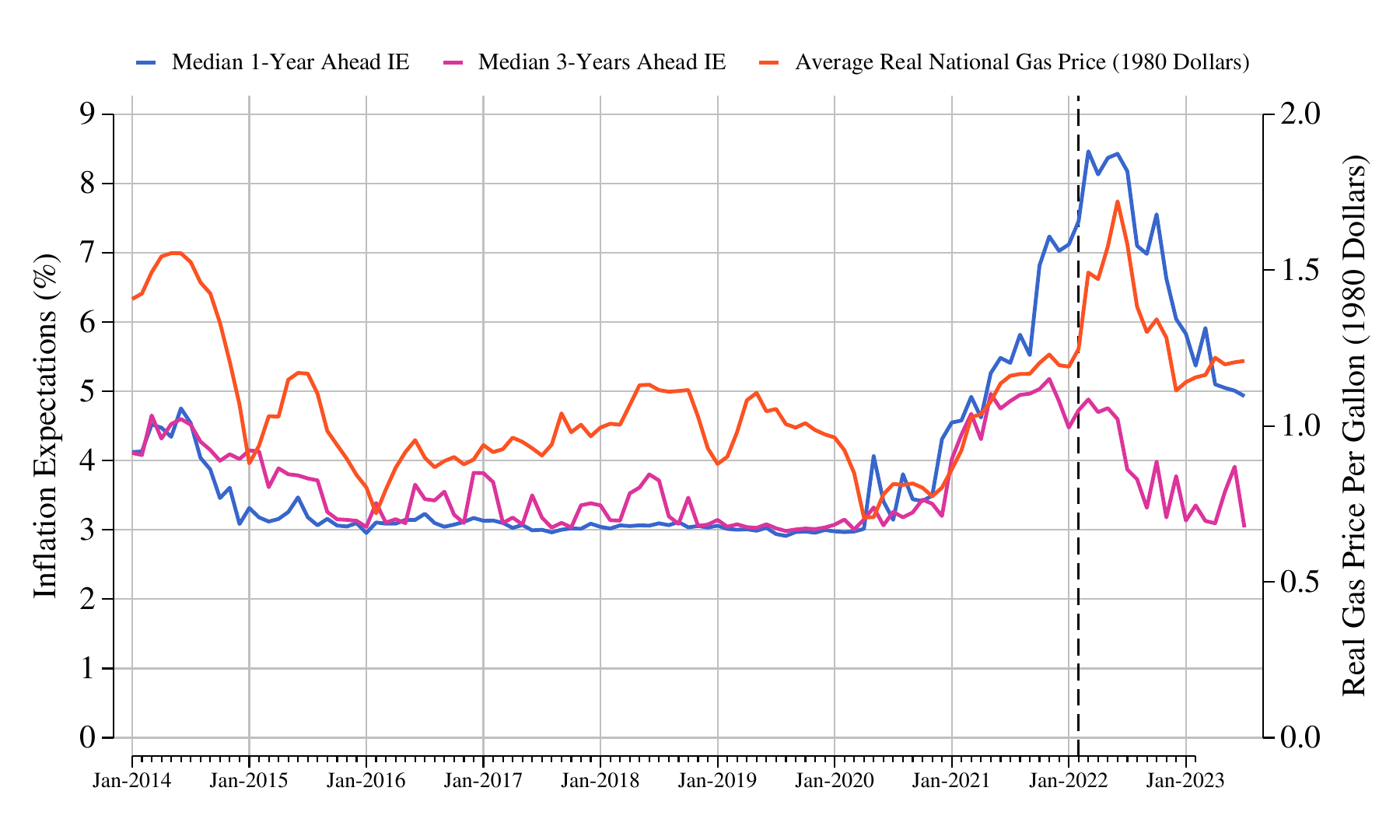
**Figure A1. Inflation Expectations and Real Gas Prices**
\
**Notes**: Median inflation expectations come from the New York Fed Survey of Consumer Expectations. Average U.S. unleaded regular gasoline prices are obtained from the U.S. Bureau of Labor Statistics. The vertical line indicates the start of Russia’s invasion of Ukraine.
**Figure A2. Year Over Year Gasoline Price Inflation from 1973 to 2023**
\
**Notes**: Average U.S. unleaded regular gasoline prices are obtained from the U.S. Bureau of Labor Statistics.
## Appendix B. Computation of counterfactual inflation expectations
The data generating process for inflation expectations in our analysis is: $$
\Delta \Pi_{t+12,t}^e = \alpha^{+} \Delta \Pi^g_{t,t-12}\cdot I\Bigl(\Delta \Pi^g_{t,t-12}\geq 0\Bigr) +
\alpha^{-} \Delta \Pi^g_{t,t-12}\cdot I\Bigl(\Delta \Pi^g_{t,t-12} < 0\Bigr) + \Omega_t
$$ where $\Delta \Pi_{t+12,t}^e$ represents the monthly change in the one-year ahead expected rate of inflation, $\Delta \Pi^g_{t,t-12}$ the change in past-year realized gas price inflation, $I(\cdot)$ represents the indicator function and $\Omega_t$ represents the residual determinant of the monthly fluctuations in inflation expectations.
Using the experimental estimates of the sensitivity of inflation expectations to positive and negative gas price changes, resp. $\alpha^{+}$ and $\alpha^{-}$, and monthly SCE core inflation expectations, we then compute the residuals $\Omega_t$ for each month after base period $b$, which in our case is February 2022.
Starting in period $b+1$ we then compute counterfactual inflation expectations $\tilde {\Pi}^e$, corresponding to a hypothetical gas price change series $\tilde {\Pi}^g$ as:
$$
\tilde {\Pi}_{b+13,b+1}^e =
\Pi_{b+12,b}^e + \alpha^{+} \Bigl[
\tilde {\Pi}^g_{b+1,b-11} -
\Pi^g_{b,b-12} \Bigr] \tilde {I^+} + \alpha^{-} \Bigl[ \tilde {\Pi}^g_{b+1,b-11} - \Pi^g_{b,b-12} \Bigr] \tilde {I^-}
+ \Omega_{b+1}
$$ where $I^+$ and $I^-$ respectively are indicators for whether the preceding term in brackets, representing the change in past-year gas price inflation, is respectively positive or negative.
Similarly for period $b+2$: $$
\tilde {\Pi}_{b+14,b+2}^e =
\tilde {\Pi}_{b+13,b+1}^e + \alpha^{+} \Bigl[
\tilde {\Pi}^g_{b+2,b-10} -
\tilde {\Pi}^g_{b+1,b-11} \Bigr] \tilde {I^+} + \alpha^{-} \Bigl[ \tilde {\Pi}^g_{b+2,b-10} - \tilde {\Pi}^g_{b+1,b-11} \Bigr] \tilde {I^-}
+ \Omega_{b+2}
$$
Through substitution for any $j=2,3,4,...$ counterfactual inflation expectations can then be computed as: $$
\tilde {\Pi}_{b+12+j,b+j}^e =
\Pi_{b+12,b}^e + \sum_{k=1}^j \alpha^{+} \Bigl[
\tilde {\Pi}^g_{b+k,b+k-12} -
\tilde {\Pi}^g_{b+k-1,b+k-13} \Bigr] \tilde {I^+} + \sum_{k=1}^j \alpha^{-} \Bigl[ \tilde {\Pi}^g_{b+k,b+k-12} - \tilde {\Pi}^g_{b+k-1,b+k-13} \Bigr] \tilde {I^-}
+ \sum_{k=1}^j \Omega_{b+k}
$$
In case of a scenario where gas prices $P^g_t$ remain constant at $P^g_b$, the assumed path for gas prices is: $$\begin{aligned}
\tilde {\Pi}^g_{b+k,b+k-12} &=& \Bigl( \frac{P^g_b - P^g_{b+k-12}}{P^g_{b+k-12}}\Bigr) \cdot 100 \ \ \ if\ k<12 \\
&=& 0 \ \ \ \ \ \ \ \ \ \ \ \ \ \ \ \ \ \ \ \ \ \ \ \ \ \ \ \ \ \ \ \ \ \ \ \ if\ k \geq 12
\end{aligned}$$ In case where the counterfactual scenario for gas prices is a 2% monthly decline after period $b$, then $$\begin{aligned}
\tilde {\Pi}^g_{b+k,b+k-12} &=& \Bigl( \frac{(P^g_b (1-0.02)^k - P^g_{b+k-12}}{P^g_{b+k-12}}\Bigr) \cdot 100 \ \ \ \ \ \ if\ k<12 \\
&=& \Bigl(1-0.02\Bigr)^{11}-1 \ \ \ \ \ \ \ \ \ \ \ \ \ \ \ \ \ \ \ \ \ \ \ \ \ \ \ \ \ \ \ \ \ if\ k \geq 12
\end{aligned}$$
## References
Aastveit, Knut Are, Bjornland Hilde C., and Jamie L. Cross. 2023. “Inflation Expectations and the Pass-Through of Oil Prices.” *The Review of Economics and Statistics* 105 (3): 733–43.
Ameriks, John, Joseph Briggs, Andrew Caplin, Minjoon Lee, Matthew D Shapiro, and Christopher Tonetti. 2020. “Older Americans Would Work Longer If Jobs Were Flexible.” *American Economic Journal: Macroeconomics* 12 (1): 174–209.
Ameriks, John, Joseph Briggs, Andrew Caplin, Matthew D Shapiro, and Christopher Tonetti. 2020. “Long-Term-Care Utility and Late-in-Life Saving.” *Journal of Political Economy* 128 (6): 2375–451.
Ameriks, John, Andrew Caplin, Steven Laufer, and Stijn van Nieuwerburgh. 2011. “The Joy of Giving or Assisted Living? Using Strategic Surveys to Separate Bequest and Precautionary Motives.” *Journal of Finance* 66 (2): 519–61.
Anderson, Soren, Ryan Kellogg, and James Sallee. 2013. “What Do Consumers Believe about Future Gasoline Prices?” *Journal of Enviromental Economics and Management* 66: 383–403.
Andre, Peter, Carlo Pizzinelli, Christopher Roth, and Johannes Wohlfart. 2022. “Subjective Models of the Macroeconomy: Evidence from Experts and a Representative Sample.” *The Review of Economic Studies* 89 (6): 2958–91. .
Armantier, Olivier, Gizem Koşar, Rachel Pomerantz, et al. 2021. “How Economic Crises Affect Inflation Beliefs: Evidence from the Covid-19 Pandemic.” *Journal of Economic Behavior & Organization* 189: 443–69.
Armantier, Olivier, Argia Sbordone, Giorgio Topa, Wilbert Van der Klaauw, and John C Williams. 2022. “A New Approach to Assess Inflation Expectations Anchoring Using Strategic Surveys.” *Journal of Monetary Economics* 129(S): 82–101.
Armantier, Olivier, Giorgio Topa, Wilbert Van der Klaauw, and Basit Zafar. 2017. “An Overview of the Survey of Consumer Expectations.” *Economic Policy Review* 23 (2): 51–72.
Armona, Luis, Andreas Fuster, and Basit Zafar. 2018. “Home Price Expectations and Behaviour: Evidence from a Randomized Information Experiment.” *Review of Economic Studies* 86 (4): 1371–410. .
Ball, Laurence, and David Romer. 1990. “Real Rigidities and the Non-Neutrality of Money.” *Review of Economic Studies* 57: 183–203.
Beshears, John, James J. Choi, David Laibson, Brigitte C. Madrian, and Stephen P. Zeldes. 2014. “What Makes Annuitization More Appealing?” *Journal of Public Economics* 116: 2–16. .
Binder, Carola. 2018. “Inflation Expectations and the Price at the Pump.” *Journal of Macroeconomics* 58: 1–18.
Binder, C, and C Makridis. 2022. “Stuck in the Seventies: Gas Prices and Macroeconomic Expectations.” *Review of Economics and Statistics* 104: 293–305.
Blanchard, O. J., and J. Galı. 2010. “The Macroeconomic Effects of Oil Price Shocks: Why Are the 2000s so Different from the 1970s?” In *International Dimensions of Monetary Policy*, edited by Gali Jordi and Mark Gertler. .
Blanchard, O. J., and M. Riggi. 2013. “Why Are the 2000s so Different from the 1970s? A Structural Interpretation of Changes in the Macroeconomic Effects of Oil Prices.” *Journal of the European Economic Association* 11 (5): 1032–52.
Christelis, Dimitris, Dimitris Georgarakos, Tullio Jappelli, Luigi Pistaferri, and Maarten van Rooij. 2019. “Asymmetric Consumption Effects of Transitory Income Shocks.” *The Economic Journal* 129 (622): 2322–41. .
Coibion, Olivier, and Yuriy Gorodnichenko. 2015. “Is the Phillips Curve Alive and Well After All? Inflation Expectations and the Missing Disinflation.” *American Economic Journal: Macroeconomics* 7 (1): 197–232.
Cover, Jame. 1992. “Asymmetric Effects of Positive and Negative Money-Supply Shocks.” *Quarterly Journal of Economics* 107 (4): 1261–82.
D’Acunto, Francesco, Ulrike Malmendier, and Michael Weber. 2023. “What Do the Data Tell Us about Inflation Expectations?” In *Handbook of Economic Expectations*. Elsevier.
Duffy, John, and Daniela Puzzello. 2014. “Experimental Evidence on the Essentiality and Neutrality of Money in a Search Model.” In *Research in Experimental Economics*. Emerald Group Publishing Limited.
Fehr, Ernst, and Jean-Robert Tyran. 2001. “Does Money Illusion Matter?” *American Economic Review* 91 (5): 1239–62.
Fuster, Andreas, Greg Kaplan, and Basit Zafar. 2021. “What Would You Do with \$500? Spending Responses to Gains, Losses, News and Loans.” *The Review of Economic Studies* 88 (4): 1760–95.
Fuster, Andreas, and Basit Zafar. 2023. “Survey Experiments on Economic Expectations.” In *Handbook of Economic Expectations*. Elsevier.
Jappelli, Tullio, and Luigi Pistaferri. 2014. “Fiscal Policy and MPC Heterogeneity.” *American Economic Journal: Macroeconomics* 6 (4): 107–36. .
Kilian, Lutz, and Xiaoqing Zhou. 2022a.“ Prices, Gasoline Prices and Inflation Expectations.” *Journal of Applied Econometrics* 37 (5): 867–81.
Kilian, Lutz, and Xiaoqing Zhou. 2022b. “The Impact of Rising Oil Prices on U.S. Inflation and Inflation Expectations in 2020–23.” *Energy Economics* 113.
Kilian, Lutz, and Xiaoqing Zhou. 2023a. “A Broader Perspective on the Inflationary Effects of Energy Price Shocks.” *Energy Economics* 125.
Kilian, Lutz, and Xiaoqing Zhou. 2023b. “Oil Price Shocks and Inflation.” In *Handbook of Inflation*.
Lusardi, Annamaria, and Olivia S. Mitchell. 2007. “Baby Boomer Retirement Security: The Roles of Planning, Financial Literacy, and Housing Wealth.” *Journal of Monetary Economics* 54 (1): 205–24.
Malmendier, Ulrike, and Stefan Nagel. 2016.“ Learning from Inflation Experiences.” *The Quarterly Journal of Economics* 131 (1): 53–87.
Mester, Loretta J. 2022. *The Role of Inflation Expectations in Monetary Policymaking: A Practitioner’s Perspective*.
Noussair, Charles, G Richter, and Jean-Robert Tyran. 2012. “Money Illusion and Nominal Inertia in Experimental Asset Markets.” *Journal of Behavioral Finance* 13 (1): 27–37.
Reis, Ricardo. 2022. *The Burst of High Inflation in 2021–22: How and Why Did We Get Here?* Working Paper No. 1060. BIS.
Roth, Christopher, Mirko Wiederholt, and Johannes Wohlfart. 2023. *The Effects of Monetary Policy: Theory with Measured Expectations*. Working Paper No. 10216. Working Paper Series. CESifo. .
Van der Klaauw, Wilbert, Wändi Bruine de Bruin, Giorgio Topa, Simon Potter, and Michael F Bryan. 2008. *Rethinking the Measurement of Household Inflation Expectations: Preliminary Findings*. SSRN Working Paper No. 1320196.
Wong, B. 2015. “Do Inflation Expectations Propagate the Inflationary Impact of Real Oil Price Shocks?: Evidence from the Michigan Survey.” *Journal of Money, Credit and Banking* 47 (8): 1673–89.
[^1]: We thank participants at the Theory and Experiments in Monetary Economics (TEME) Conference 2022. We also thank John Duffy, Rod Garatt and Damjan Pjafar for useful comments. We are grateful to the editor and two anonymous referees for their help in improving the manuscript. Finally, we would like to thank Jasmina Arifovic whose work, advice and kindness has been an inspiration. The opinions expressed herein are those of the authors and not necessarily those of the Federal Reserve Bank of New York or the Federal Reserve System.
[^2]: Federal Reserve Bank of New York.
[^3]: The influence of crude oil prices on IE was also established by e.g. (Blanchard and Galı 2010), (Blanchard and Riggi 2013) or (Wong 2015). Note that our paper focuses on gasoline prices consumers pay at the pump, not crude oil nor natural gas prices.
[^4]: , retrieved on October 22, 2023.
[^5]: , retrieved on October 22, 2023. Mary Daly, President of the Federal Reserve Bank of San Francisco, also stated in April 2022: “*Long periods of high inflation, even if it is projected to come down, can seep into expectations, leading people to anticipate further price increases. This is especially salient now, with prices for food and gasoline making headlines. Research tells us that these prices heavily influence consumers’ beliefs about future inflation*.” , retrieved on October 22, 2023.
[^6]: , retrieved on October 22, 2023.
[^7]: The SCE questionnaire design followed an extended testing and experimentation phase between 2006 and 2012 that used in-depth cognitive interviews, psychometric surveys and various pilot surveys. This testing phase is documented in (Van der Klaauw et al. 2008) and (Armantier et al. 2017).
[^8]: Similarly, one-year ahead median IE in the Michigan Survey of Consumers rose from 2.5% in January 2020 to a peak of 5.4% in April 2022, followed by a tapering off to 3.4% in July 2023. Long-term (five- to ten-year ahead) median IE in the Michigan Survey of Consumers increased from 2.5% in January 2020 to 3.1% in June 2022, after which it declined to 3.0% in July 2023.
[^9]: Figure [A1](#fig:ie_gas_prices_real) in Appendix shows a similar spike when gasoline prices are expressed in real terms.
[^10]: Over the entire history of the SCE the correlation between gasoline prices and median short-term IE is 0.81, while the correlation is 0.41 for monthly changes, and 0.76 for yearly changes in these variables. Over the entire history of the SCE the correlation between gasoline prices and median medium-term IE is 0.62, while the correlation is 0.17 for monthly changes, and 0.44 for yearly changes in these variables.
[^11]: The “positive food price shock” treatment asks respondents: *Suppose that if instead of increasing by about 8%, food prices had instead risen by 12% over the last 12 months*. Note that the actual price growth for gasoline, food and durables was indeed about 40%, 8% and 12% during the 12 months that preceded the experiment. The magnitude of the hypothetical price shocks (50%) was chosen as a compromise between saliency and realism. In particular, Figure [A2](#fig:gas_inflation) in Appendix shows that a 50% gasoline price inflation, although rare, has occurred on occasion since the 1970s, including in several months between 2021 and 2022.
[^12]: While we recognize the value of randomizing the order in which treatments are presented, we decided to keep them fixed i) to facilitate comparisons across respondents and ii) so that we can pool gasoline price revisions across experiments in the subsequent analysis.
[^13]: For example, the increase in gasoline prices in 2021 and part of 2022 coincided with pandemic-related supply chain disruptions, a rise in economic uncertainty (extending beyond the war in Ukraine), and an increase in aggregate demand which led to increases in the prices of most goods and services. This makes it difficult to isolate precisely the role played by gasoline prices in the increase in IE.
[^14]: For instance, an actual 50% gasoline price shock may be incorrectly perceived by consumers as a larger shock because it may be amplified through media reports or purchase frequency. In that case, our experiment should be interpreted as measuring the impact of *perceived* (rather than *actual*) 50% price shocks.
[^15]: See also (Ameriks et al. 2011), (Beshears et al. 2014), (Jappelli and Pistaferri 2014), (Christelis et al. 2019), (Ameriks, Briggs, Caplin, Lee, et al. 2020), (Fuster et al. 2021), (Fuster et al. 2021), (Fuster and Zafar 2023), (Roth et al. 2023).
[^16]: One may be concerned that zero revisions reflect inertia, fatigue or a lack of effort in answering the questions. We find no evidence to support this hypothesis. In particular, non-revisers took essentially as much time to complete the survey as non-revisers. Further, the substantial differences in the proportions of non-revisers across treatments in Figure 2 suggest that these responses are deliberate and informative.
[^17]: See also Tables [A2](#tab:gasrevdemo1) and [A3](#tab:gasrevdemo3) in Appendix for average normalized revisions in each demographic group.
[^18]: This is the case in our survey as well. The median IE of respondents 55 and older are 8.1% and 5.2% at the one- and three-year horizons, as compared to 5.7% and 3.6% for those below the age of 35, and 6.5% and 4.2% for those between the age of 35 and 55.
[^19]: In related work, (Binder and Makridis 2022) find that the sentiment of older consumers about the economy declines more than their peers when gasoline prices rise.
[^20]: (Binder 2018) uses gasoline expenditure share of 4 to 5%, which would lead to ratios even closer to the one we obtained in the positive shock treatment.
[^21]: (Kilian and Zhou 2022a) observe that if gasoline price expectations follow a random walk (as suggested by e.g. Anderson et al. (2013)), then gasoline price shocks should have no impact on IE. In that case, any sensitivity of IE to gasoline prices should be considered excessive.
[^22]: (Kilian and Zhou 2022a) show that the link between gasoline prices and IE is time-varying. Therefore, although we run our simulation over a relatively short period of time, the second condition may not be supported empirically.
[^23]: See Appendix B for details on the implementation of the counterfactual exercise.