---
schema_version: 1
title: 'Menu-Dependent Risk Attitudes: Theory and Evidence'
authors:
- Zhuo Chen
- Russell Golman
- Jason Somerville
language: en
edition: Author manuscript · October 2023
date: '2023-10-25'
paper_url: https://jason-somerville.com/papers/menu-dependent-risk-attitudes/
pdf_url: https://jason-somerville.com/files/menu-dependent-risk-attitudes/paper.pdf
format: Markdown with TeX mathematics
---

# Menu-Dependent Risk Attitudes: Theory and Evidence

Zhuo Chen, Russell Golman, and Jason Somerville

*October 25, 2023*

## Abstract

We test for a novel pattern of menu-dependent risk attitudes that forms the basis of recent theories of risky choice: Does expanding the range of potential prizes from lotteries in a choice set lead people to overweight those prizes and make riskier choices? Contrary to our hypothesis, we find no evidence of such a menu effect. Varying the potential prize offered by an actuarially unfavorable, high-risk lottery does not affect the likelihood of choosing a different, moderate-risk gamble in favor of a safer alternative. Our well-powered null results cast doubt on prominent theories of menu-dependent risk preferences.

**Keywords:** Focusing, Menu Dependence, Risk Attitudes

**JEL codes:** C91, D81

## Introduction

Gambles offering a small chance of a substantial gain are famously appealing. Many people sink their money into lottery draws and slot machines with staggering jackpots, despite these gambles having negative expected returns. Prior work has emphasized the overweighting of small probabilities as the primary mechanism for this risk-seeking behavior when evaluating highly skewed gambles (Kahneman and Tversky 1979; Tversky and Kahneman 1992). However, some people are drawn into the casino by the allure of the large jackpot only to take a seat at the roulette table, choosing a different gamble with smaller potential winnings but a somewhat better expected return. Many risky decisions outside the casino also involve a range of potentially extreme outcomes, which may attract attention and affect risk attitudes. The possibility of investing in bitcoin might affect an investor who is choosing between an index fund or a bond fund. The option to start a business might influence a candidate’s decision between a job with more stability or one with more potential for advancement. The prospect of going without insurance altogether could affect the choice of a health insurance deductible. Given the prevalence of such extreme options in many high-stakes financial decisions, it is important to understand how they shape individuals’ risk tolerance.

Both prospect theory and expected utility theory rule out the possibility that the range of possible outcomes in the choice set could affect risk attitudes because they both satisfy the property of independence of irrelevant alternatives (IIA). Nevertheless, the tendency to focus on specific aspects of a decision based on features of the available alternatives is well accepted in psychology (Schkade and Kahneman 1998) and has recently been incorporated into choice models in economics (Bordalo et al. 2012; Kőszegi and Szeidl 2013; Gabaix 2019). These theories have sought to relax the IIA assumption by allowing preferences to depend on the entire menu of options under consideration. The primary psychological intuition at the heart of models of menu-dependent risk attitudes is that the range of outcomes across lotteries in a menu affects the attention allocated to these outcomes and thus affects choices between these lotteries. Menu-dependent risk attitudes can shed light on empirical results that are inconsistent with both expected utility theory and menu-independent non-expected-utility models, such as context-dependent choice reversals (Lichtenstein and Slovic 1971; Tversky et al. 1990). While this approach is promising, theory-based experiments are needed to test the specific menu-dependent risky choice patterns central to these new theories.

This paper presents an experiment that tests a prominent hypothesized pattern of menu-dependent risk attitudes. We explore whether individuals’ willingness to take on risk associated with an actuarially favorable lottery depends on the risk profile of a different, actuarially unfavorable lottery in the menu. The basic intuition we test is whether expanding the range of potential upside of the lotteries in the choice set causes people to overweight each lottery’s upside and thus take on more risk. The tendency to overweight attributes or outcomes that vary more widely is the primary assumption in the focusing model of Kőszegi and Szeidl (2013) and closely related to the ordering property in salience theory (Bordalo et al. 2012).

Contrary to our hypotheses, we find no evidence of this pattern of menu-dependent risk attitudes. We show that varying the skewness (and variance) of an unfavorable, rarely chosen high-risk lottery does not alter the likelihood of choosing a moderate-risk gamble over a safer alternative. When this high-risk lottery is highly skewed, it offers a large potential prize, albeit with a very low probability; as it becomes less skewed, the range of possible prizes in the menu narrows. However, the expected-value premium required to induce choices of the moderate-risk gamble over the safe alternative remains unaffected by this variation of the high-risk lottery. Removing the high-risk option from the choice set entirely does not alter the relative demand shares of the remaining options. This evidence is inconsistent with focusing and the broader notion that altering the distribution of outcomes in the choice set systematically impacts individuals’ risk attitudes. In contrast, we cannot reject expected utility with heterogeneous risk attitudes and choice noise or models of probability weighting (Kahneman and Tversky 1979; Quiggin 1982; Tversky and Kahneman 1992).

A key challenge when applying models of menu-dependent risk attitudes is defining the relevant attributes. To motivate our experimental tests, we develop a theoretical framework that draws on the key intuition of focusing (Kőszegi and Szeidl 2013) and salience theory (Bordalo et al. 2012).[^1] In this model, agents’ focus is drawn to either the upside or the downside of the lotteries in the choice set based on the relative range of outcomes on each side. We show that for simple lotteries with two outcomes, this specification of menu-dependent risk attitudes leads to straightforward distinguishing predictions relative to menu-independent models. We consider a context in which individuals choose between three lotteries: a safe, a moderate-risk, and a high-risk option. The key comparative static of our model is that increasing the skewness of the payoffs for the high-risk lottery leads to more risk-seeking behavior even if individuals never choose the high-risk lottery; that is, more choices of the moderate-risk lottery in favor of the safe alternative.

We designed and implemented an experiment to test the distinguishing comparative static predictions that we derived from focusing theory applied to risky choice. In our main experimental task, we asked participants to choose their preferred option from a full menu containing a safe, a moderate-risk, and a high-risk option. Each option was a simple lottery that offered a monetary prize with some probability and zero otherwise. The moderate-risk option had an expected-value surplus relative to the safe option indexed by the parameter $\beta$. The high-risk option had a lower expected value than the safe option but had the highest potential prize. The parameter $\alpha$ inversely indexed the skewness of high-risk option, hence the range of the upside in the choice set. Our central experimental manipulation was to vary both the expected-value surplus $\beta$ and the skewness parameter $\alpha$ in a within-subjects design. These manipulations allow us to test whether the expected-value surplus participants require to take on moderate risk is affected by the range of upside outcomes – specifically, whether it is an increasing function of $\alpha$.

We find no evidence that risk-taking is dependent on menu composition. The likelihood of choosing a moderate-risk option over a safe option is unaffected by the skewness of the high-risk lottery. The expected-value surplus that participants demand to take on risk is independent of the upside range. Removing the high-risk option from the menu entirely has no impact on the fraction of risky choices. Conversely, we find that participants clearly respond to the expected-value surplus. When the safe and moderate-risk options had the same expected value, the demand shares were 66% and 18%, respectively. However, when the moderate-risk option had an expected value twice as large as the safe option, only 49% chose the safe option, while 40% chose the moderate-risk option. The fact that participants did respond to this experimental variation rules out inattention or random choice as an explanation for our null finding.[^2] The absence of a prize-range effect casts doubt on the focusing model of menu-dependent risk attitudes in our study context and provides new empirical evidence to guide refinements to menu-dependent models of choice under risk.

Our data contain rich within-person variation, allowing us to explore heterogeneity in risk attitudes across participants. Around 21% of participants were highly risk averse; that is, they always chose the safe option from the full menu in all 36 choices, foregoing a moderately risky alternative with up to twice the expected value. Most participants were moderately risk averse: roughly 57% of participants switched between the safe and moderate-risk options depending on the magnitude of the expected surplus premium. The remaining share of participants were, at times, risk-seeking in the sense that they chose the high-risk option several times despite its inferior expected value and higher risk. These participants were likelier to switch to the high-risk option when we presented them with more skewed payoffs. These risk attitudes are consistent with expected utility with heterogeneous risk attitudes as well as with models of probability weighting.

We contribute to a growing literature that tests the predictions of theories of menu dependence in risky choice. The absence of menu effects in our three-option choice sets is a puzzle in light of previous findings from binary choice settings. This existing literature has mainly focused on testing the predictions of salience theory (Bordalo et al. 2012) in menus with just two options. Frydman and Mormann (2018) find that increasing the correlation between payoffs across lotteries leads to a reduction in common-consequence violations. They also show that including an unavailable option in the menu doubles the number of common-consequence violations. These results are consistent with salience theory but inconsistent with expected utility theory and cumulative prospect theory. Dertwinkel-Kalt and Köster (2020) show that participants respond to the relative skewness of lotteries in a manner consistent with salience theory. Similarly, Nielsen et al. (2021) find that people are more likely to allocate money to riskier lotteries when the good outcomes of those lotteries are more salient. In contrast, Alós-Ferrer and Ritschel (2022) find that the presence of an alternative option does not reduce the rate of preference reversals in a manner consistent with salience theory.[^3] Our results also cast doubt on whether a central intuition of salience theory is an empirically relevant force in a different context.

We emphasize that our results do not imply that the IIA axiom holds more generally. Other menu effects, such as asymmetric dominance, have been documented in previous experiments investigating choice under risk (Herne 1999; Soltani et al. 2012; Farmer et al. 2017). Range effects in risky choice have been found in other contexts, although these effects sometimes run in opposite directions. Simonson and Tversky (1992) find that adding an extreme option to the choice set generates a polarization effect in risky choice while Herne (1999) finds an opposite compromise effect. Castillo (2020) shows that adding symmetrically dominated decoy lotteries to the choice set leads to range effects. Our results also add to previously mixed evidence on focusing in other domains. Dertwinkel-Kalt et al. (2022) find that individuals are willing to work more to receive concentrated payments in a single period consistent with focusing (Kőszegi and Szeidl 2013). In the domain of riskless consumer choice, Somerville (2022) documents robust evidence supporting the relative-thinking model (Bushong et al. 2021), which makes the opposite predictions of focusing. Contrary to these findings for riskless choice, we find a complete absence of range effects in risky choice. Our results highlight the need for further empirical evidence to establish the contexts in which IIA violations do and do not occur and the mechanisms that drive such effects.

The rest of this paper is organized as follows. Section 2 introduces our theoretical framework and derives the key comparative statics we test. Section 3 describes the design and implementation of our experiment. Section 4 presents our main results and an individual heterogeneity analysis. Section 5 considers the implications of our results for alternative theories of risk preferences. Section 6 further discusses our findings and concludes.

## Theoretical Framework

In this section, we introduce a general framework of menu-dependent risk attitudes over simple lotteries. We illustrate how menu dependence can shape risk attitudes and account for both risk- averse and risk-seeking behavior. We also derive novel, distinguishing predictions of the model that guide our experimental design and empirical analyses

### A Model of Menu-Dependent Risk Attitudes

Consider an agent that faces a choice between simple lotteries of the form $x = (z_1,z_2; p)$ that offer prize $z_1 \in \mathbb{R}$ with probability $p$ and prize $z_2 \in \mathbb{R}$ with probability $1-p$, where $z_1 > z_2$. We assume that agents frame each lottery in terms of its potential *upside* and *downside*. The potential upside is a lottery’s best outcome, $\overline{z}(x)=z_1$. The potential downside is its worst outcome, $\underline{z}(x)=z_2$.[^4] We use $\delta_z$ to denote a lottery that pays out $z$ with certainty and assume that $\overline{z}(\delta_z) = \underline{z}(\delta_z) = z$.

The agent’s focus is drawn to either the upside or downside of a lottery based on the composition of the menu. Let $\mathcal{C}$ denote the consideration set.[^5]

Then, the utility of lottery $x$ is given by,

$$
V(x;\mathcal{C})=w(p;\mathcal{C}) u(z_1)+[1-w(p;\mathcal{C})] u(z_2), \tag{1}
$$

where $u$ is a utility function for money and $w(p;\mathcal{C})\in[0,1]$ is the menu-dependent weight that the agent places on upside prize. Expected Utility Theory (EUT) is nested in this specification and corresponds to $w(p;\mathcal{C}) = p$.

Our notion of menu dependence draws on the intuition at the heart of the focusing model of Kőszegi and Szeidl (2013) and the salience theory of Bordalo et al. (2012), which proposes that people overweight attributes that vary the most in the choice set. In our context, the attributes that matter are the upside and downside prizes of the lotteries in the menu. We assume that the relative range of possible outcomes along these dimensions determines the weight that agents place on each outcome. Specifically, we assume that the decision weight that agents assign to the upside outcome is,

$$
w(p;\mathcal{C})=\frac{p \; g\left(\overline{\Delta}(\mathcal{C})\right)}{p \; g\left(\overline{\Delta}(\mathcal{C})\right) +(1-p) \; g\left(\underline{\Delta}(\mathcal{C})\right)}, \tag{2}
$$

where $\overline{\Delta}(\mathcal{C})=\max_{x\in \mathcal{C}}\overline{z}(x)-\min_{x\in \mathcal{C}}\overline{z}(x)$ is the upside range, $\underline{\Delta}(\mathcal{C})=\max_{x\in \mathcal{C}}\underline{z}(x)-\min_{x\in \mathcal{C}}\underline{z}(x)$ is the downside range, and $g$ is strictly increasing in $\Delta$ and strictly positive. This implies that the weight attached to the upside of a lottery is increasing in the range of possible upside payoffs. For example, consider menus $\mathcal{C}_1$ and $\mathcal{C}_2$ such that $\underline{\Delta}(\mathcal{C}_1)=\underline{\Delta}(\mathcal{C}_2)$ but $\overline{\Delta}(\mathcal{C}_1)>\overline{\Delta}(\mathcal{C}_2)$. Agents will focus more on the upside of the lotteries in $\mathcal{C}_1$ than in $\mathcal{C}_2$, and therefore agents will weight the upsides of the lotteries more in $\mathcal{C}_1$ than in $\mathcal{C}_2$, that is, $w(p;\mathcal{C}_1)>w(p;\mathcal{C}_2)$.

Equation (2) implies that the upside prize is overweighted if and only if $\overline{\Delta}>\underline{\Delta}$. However, since $u$ can be concave or convex, agents can still be risk averse or risk seeking when $\overline{\Delta}=\underline{\Delta}$. More generally, for lotteries $x=(z_1,z_2;p)$ and $x'=(z'_1,z'_2;p')$ where $z'_1>z_1>z_2>z_2'$ and $pu(z_1)+(1-p)u(z_2)=p'u(z'_1)+(1-p')u(z'_2)$, $x$ is preferred to $x^\prime$ if and only if $\overline{\Delta}\leq\underline{\Delta}$. In other words, people are more risk averse when they are downside focused and more risk seeking when they are upside focused. In the extreme, if $g\left(\overline{\Delta}(\mathcal{C})\right)/ g\left(\underline{\Delta}(\mathcal{C})\right)\rightarrow\infty$, then agents are completely upside focused and simply maximize $u(\overline{z}(x))$. Conversely, if $g\left(\overline{\Delta}(\mathcal{C})\right)/ g\left(\underline{\Delta}(\mathcal{C})\right)\rightarrow0$, then agents are entirely downside focused and will maximize is $u(\underline{z}(x))$. In practice, we assume that $g(0)>0$ and $\lim_{\Delta \rightarrow \infty}g(\Delta)<\infty$ so that agents will always place some weight on both the upside and the downside of the lotteries in the menu whenever $p\in(0,1)$.

To illustrate the role that the menu composition plays in shaping risk attitudes, consider an agent who is deciding between a risky lottery $x$ and a sure payment equal to the expected value of that lottery, $\delta_{EV(x)}$. To isolate the role of menu dependence in risky choice, we assume that utility for money is linear, $u(z) = z$. Given choice set $\mathcal{C} = \{x,\delta_{EV(x)}\}$, the range of potential upsides is $\overline{\Delta}(\mathcal{C}) = (1-p)(z_1 - z_2)$ and the range of potential downsides is $\underline{\Delta}(\mathcal{C}) = p(z_1 - z_2)$. Holding fixed the expected value of $x$ and the lowest outcome $z_2$, increases in $z_1$ must be offset by decreases in $p$. As $z_1$ gets larger and $p$ gets smaller, agents’ focus is drawn toward the potential upside of the lottery, inducing risk-seeking behavior. In other words, agents will prefer a lottery with a relatively small possibility of a large prize over the expected value of that lottery for certain. Conversely, hold fixed highest outcome $z_1$, and let $p$ and $z_2$ vary. Then decreases in $z_2$ will be offset by higher $p$, which expands the range of potential downside outcomes and induces risk aversion. In other words, for lotteries with a small probability of a bad outcome, agents will prefer the expected value of the lottery.

A key feature of menu dependence is that it generates a preference for skewed outcomes. Figure 1 depicts willingness to pay for a lottery with fixed outcomes $z_1$ and $z_2$ as a function of $p$. Willingness to pay has a classic inverse-S shape that is typically assumed by probability weighting models (Kahneman and Tversky 1979; Quiggin 1982; Tversky and Kahneman 1992). This inverse-S shape arises endogenously under menu dependence due to focusing effects. However, as emphasized by Bordalo et al. (2012), menu dependence need not generate overweighting of small probabilities. For example, consider menu $\mathcal{C}=\{x,x^\prime\}$ where $x=(z_1,z_2;1-p)$ and $x'=(z'_1,z_2;1-p')$, $EV(x)=EV(x')$, and both $p$ and $p'$ are close to $0$ with $p>p^\prime>0$. Then, the upside range is $\overline{\Delta}(\mathcal{C})=(p-p^\prime)(z_1-z_2)/(1-p') > 0$, and the downside range is $\underline{\Delta}=0$. As $g$ is a strictly increasing function, focusing therefore implies that both $p$ and $p'$ are underweighted.

<a id="fig:wtp_fig"></a>

![Figure wtp_fig](assets/wtp-graph.png)

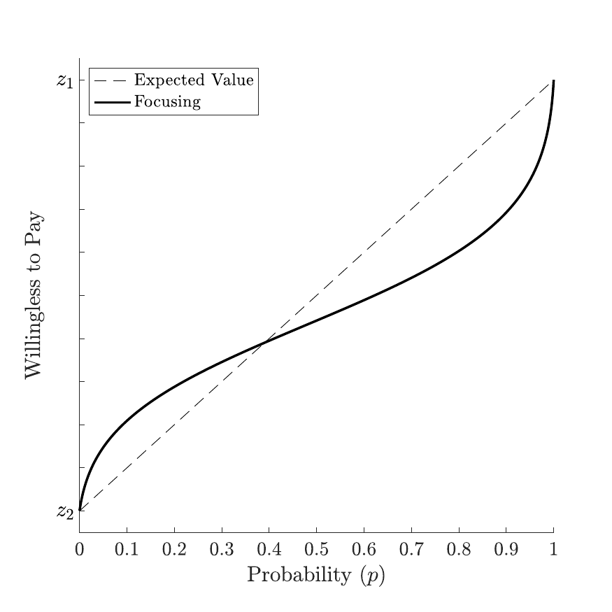
 Figure 1: The solid black line denotes willingness to pay for lottery $x = (z_{1}, z_{2}; p)$ under menu-dependent attribute weighting. The consideration set is $\mathcal{C} = \{x, \delta _{m}\}$ and willingness to pay is the value of $m$ such that focusing agents are indifferent between the two options. The attribute weighting function is $g(\Delta ) = \exp \{\gamma (\Delta - k)/(\Delta + k)\}$ and the utility function for money is $u(y) = - \exp \{- ry\}$. The parameter values are $\gamma = 2.5$, $k = 5$ and $r = 0.2$ and the outcomes are $z_{1} = 2z_{2} = 10$. The dashed line denotes willingness to pay under expected value maximization.

Menu dependence can help account for a number of behavioral regularities that cannot be explained by EUT. Focusing can cause agents to overweight both good and bad low-probability outcomes. Thus, it can account for the observation that people buy lottery tickets and insurance simultaneously. In Appendix B, we demonstrate that menu dependence can account for the common-ratio effect (Kahneman and Tversky 1979; Blavatskyy et al. 2020) and preference reversals (Lichtenstein and Slovic 1971). Beyond accounting for these empirical findings, menu dependence also generates novel predictions that distinguish it from both EUT and other menu-independent theories of choice under risk.

### Theoretical Predictions

In this section, we derive the main theoretical predictions that our experiment was designed to test. We leverage two features of menu dependence that lead to distinguishing comparative statics. First, focusing can generate a preference for skewed returns. As the range of potential upside expands, agents overweight the positive aspects of a gamble, which leads them to take on more risk. Second, we draw on a large literature that highlights the role that seemingly irrelevant options can play in shaping outcomes when agents have menu-dependent preferences (Huber et al. 1982; Simonson 1989; Somerville 2022). Specifically, we consider the case in which the presence of an inferior, rarely chosen lottery in the menu alters the skewness of the returns and, hence, the relative weights of the upside and downside of each lottery.

We consider lotteries of the form $x_i=(z_i,0;p_i)$ for $i = 1, 2, 3,$ where $z_1<z_2<z_3$ and $p_1>p_2>p_3$. Furthermore, we restrict attention to the following case:

$$
\begin{aligned}
 (p_1,p_2,p_3) &=\left(p,\frac{p}{2},\alpha\frac{p}{2}\right) \qquad \text{and} \\
 (z_1,z_2,z_3) &=\left(z,2\beta z,\frac{4}{3\alpha}z\right),
\end{aligned}
$$

where $z>0$, $p\in(0,1]$, $\alpha\in\left(0,2/(3\beta)\right]$, and $\beta\geq 1$. Note that for an arbitrary $(z,p)$, the parameters $\alpha$ and $\beta$ determine the relative attractiveness of the three alternatives. First, $\beta$ indexes the expected-value premium that $x_2$ offers relative to $x_1$: $EV(x_2)=\beta EV(x_1) = \beta p z$. Therefore, while $x_2$ involves more risk than $x_1$, it also offers a higher expected value that is increasing in $\beta$. Second, $\alpha$ determines the upside range whenever $x_3$ is included in the menu. Lottery $x_3$ is designed to be a highly skewed “decoy.” It is not a traditional decoy option that is strictly dominated by another option in the menu. However, it is first-order stochastically dominated by lottery $x'_3=((2\beta/\alpha)z,0;\alpha p/2)$, which is second-order stochastically dominated by $x_2$. As $x_3$ offers the lowest expected return of $EV(x_3) = (2/3) EV(x_1)$ and also carries the most risk, agents will only chose it if they are very risk seeking. Nonetheless, $x_3$ may influence the relative preference for $x_1$ versus $x_2$ by altering whether agents focus on the upside or downside of these lotteries.

Formally, suppose that agents face consideration set $\mathcal{C}(\alpha,\beta) = \{x_1,x_2(\beta),x_3(\alpha)\}$. The downside range is unaffected by the values of $\alpha$ or $\beta$ and hence the weight attached to the downside of each lottery is fixed. Conversely, the upside range is directly determined by the magnitude $\alpha$:

$$
\overline{\Delta}(\alpha) \equiv \overline{\Delta}(\mathcal{C}(\alpha,\beta))=\left(\frac{4}{3\alpha}-1\right)z
$$

As $\alpha$ decreases, $\overline{\Delta}(\alpha)$ increases with the skewness of lottery $x_3(\alpha)$. This causes agents to place a great weight on each lottery’s upside, which induces more risk-seeking behavior.

**Prediction 1.** For menu $\mathcal{C}(\alpha,\beta)$, agents are more upside focused and hence more risk seeking when $\alpha$ is smaller. That is, for any $\alpha$ and $\alpha'$ such that $\alpha<\min\{\alpha',2/(3\beta)\}$, then if $x_1$ is not chosen in $\mathcal{C}(\alpha^\prime,\beta)$, it will not be chosen in $\mathcal{C}(\alpha,\beta)$ either.

When deciding between $x_1$ and $x_2(\beta)$, menu dependence predicts that as $\alpha$ decreases, agents will be less likely to choose the relatively safe option $x_1$ over the moderate-risk option $x_2(\beta)$. Formally, let $\beta^*(\alpha)$ denote the expected-value premium such that agents are indifferent between these two options.[^6] Then, prediction 1 implies that $\beta^*(\alpha)$ is a strictly increasing function. Figure 2 plots expected value threshold, $\beta^*(\alpha)$ as a function of $\alpha$. As $\alpha$ decreases, the upside range expands which causes agents to become more risk seeking—thus, the expected-value surplus required for them to choose the risk option also decreases.

<a id="fig:exp_predictions"></a>

![Figure exp_predictions](assets/exp-prediction.png)

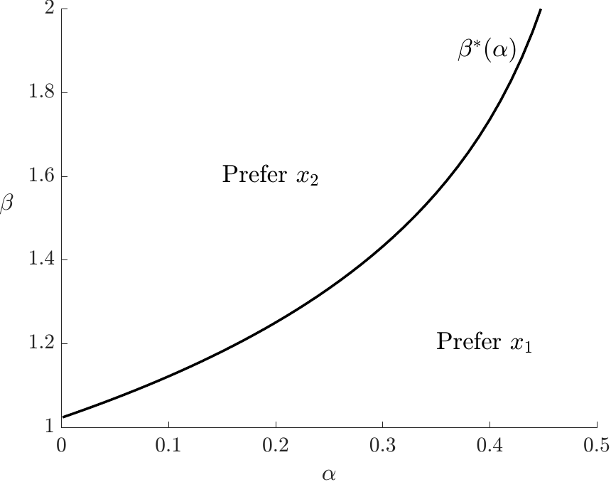
 Figure 2: Predicted choices under focusing for menu $\mathcal{C}(\alpha , \beta ) = \{x_{1}, x_{2}(\beta ), x_{3}(\alpha )\}$. $\beta$ indexes the expected-value surplus between the relatively safe option, $x_{1}$, and the moderate-risk option, $x_{2}(\beta )$. The upside range is decreasing in $\alpha$. The attribute weighting function is $g(\Delta ) = \exp \{\gamma (\Delta - k)/(\Delta + k)\}$ and the utility function for money is $u(y) = - \exp \{- ry\}$. The parameter values are $\gamma = 0.25$, $k = 5$ and $r = 0.2$, and the safest option is $x_{1} = (z, p) = (5, 1)$. The threshold $\beta ^{*}(\alpha )$ is the value of $\beta$ such that agents are indifferent between the $x_{1}$ and $x_{2}(\beta )$.

Menu dependence will exert less influence when the high-risk option $x_3(\alpha)$ is excluded from the menu. For example, when agents face the choice set $\mathcal{C}(\beta) = \{x_1,x_2(\beta)\}$, the upside range is $\overline{\Delta}(\beta) \equiv \overline{\Delta}(\mathcal{C}) = 2(\beta - 1)z$ and the downside range is 0. As a result, agents will prefer the riskier option $x_2$ over the safer option $x_1$ if and only if

$$
\frac{g\left(\overline{\Delta}(\beta)\right)}{g(0)}\geq\frac{(2-p)u(z)-(1-p)u(2\beta z)}{p(u(2\beta z)-u(z))}. \tag{3}
$$

As $\overline{\Delta}(\beta) < \overline{\Delta}(\alpha)$, this condition is harder to satisfy in menu $\mathcal{C}(\beta)$ than in menu $\mathcal{C}(\alpha,\beta)$.

**Prediction 2.** Agents are more risk seeking in menu $\mathcal{C}(\alpha,\beta)$ than in menu $\mathcal{C}(\beta)$. That is, if $x_1$ is not chosen in $\mathcal{C}(\beta)$, then it will not be chosen in $\mathcal{C}(\alpha,\beta)$ either.

Finally, we consider how menu dependence can shape risk attitudes when agents decide between the safest option $x_1$ and the high-risk option $x_3(\alpha)$. For choice set $\mathcal{C}(\alpha) = \{x_1,x_3(\alpha)\}$, the upside range is $\overline{\Delta}(\alpha)$. Therefore, smaller values of $\alpha$ induce more risk-seeking. The absence of the moderate-risk option means that greater skewness boosts the appeal of $x_3(\alpha)$ relative to $x_1$.

**Prediction 3.** For any $\alpha'>\alpha$, subjects are more upside focused and, hence, more risk seeking in menu $\mathcal{C}(\alpha)$ than in menu $\mathcal{C}(\alpha')$. That is, if $x_1$ is not chosen in $\mathcal{C}(\alpha')$, then it will not be chosen in $\mathcal{C}(\alpha)$.

Predictions 1, 2, and 3 form our main experimental hypotheses. The key assumptions underpinning these predictions are that: (i) agents frame lotteries in terms of the upside and the downside outcomes; (ii) the weight attached to a lottery’s upside is increasing in its range; (3) the upside range is increasing in $\alpha$. Alternative formulations of menu dependence will share these predictions. Thus, our experimental tests are designed to test for menu dependence in risky choice more generally. In Section 5, we relate our results to other theories of menu dependence risk attitudes.

## Experimental Design

This section describes the design and implementation of our experiment. We provide screenshots of the experimental tasks and all participant instructions in the Online Appendix.

### Choice Environment

Participants’ task was to choose their preferred option from a menu of either two or three lotteries. Each lottery paid out a prize with some probability and zero otherwise. The lotteries differed in both the prize amount and the probability of winning. There were three types of lotteries that participants saw during the experiment: a safe option, a moderate-risk option, and a high-risk option. The safe option offered prize $z>0$ with a relatively high probability $p\geq0.9$. The moderate-risk option offered a larger prize $2 \beta z$ with lower probability $p/2$, where $\beta \geq 1$. The high-risk option offered the largest prize $4z/(3\alpha)$ with a relatively low probability $\alpha p/2$, for some small $\alpha \in (0,1/\beta]$. Figure 3 presents an example choice screen from a three-option menu with $p = 1$, $z=2.2$, $\alpha = 0.2$, and $\beta = 1.4$.

<a id="fig:ex_choice"></a>

![Figure ex_choice](assets/choice-task.png)

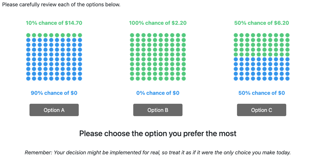
 Figure 3: Example choice task for a three-option menu with experimental parameters $p = 1$, $z = 2.2$, $\alpha = 0.2$, and $\beta = 1.4$.

Each participant made a series of choices from menus containing either two or three of these lotteries. The key experimental manipulation was to vary the values of $\alpha$ and $\beta$ across trials within subject. In our theoretical framework, the value of $\alpha$ inversely indexes the upside range in the choice set. We therefore varied the upside range by manipulating the value of $\alpha$. We set $\alpha$ equal to one of six values in each trial: $0.05$, $0.1$, $0.15$, $0.2$, $0.25$, and $0.3$. To compensate for baseline risk aversion and make the moderate-risk lottery more appealing, we also varied the expected-value premium for the moderate-risk lottery relative to the safe lottery, which is indexed by $\beta$. We set $\beta$ equal to one of six values on each trial: $1$, $1.2$, $1.4$, $1.6$, $1.8$, and $2$.

Participants chose their preferred option from three different menus for each combination of $\alpha$ and $\beta$ values. The first menu consisted of all three lotteries: the safe, moderate-risk, and high-risk options. Participants chose from this full menu in 36 trials—one for each $\alpha$-$\beta$ combination. The second menu contained just the safe and moderate-risk lotteries. Participants chose from this restricted menu in six trials—one for each value of $\beta$. The third menu contained just the safe and high-risk lotteries. Participants chose from this restricted menu in six trials—one for each value of $\alpha$. In total, participants made choices in 48 trials involving these three menus in randomized order.

On each of these 48 trials, we drew the prize of the safe option $z$ from a uniform distribution over the interval $[\$1,\$3]$. The probability of winning this prize $p$ was set to 1 with probability 1/2, 0.99 with probability 1/6, 0.95 with probability 1/6, and 0.9 with probability 1/6. The values of $p$ were counterbalanced within each kind of menu so that each participant saw $p=1$ in $18$ trials with the full menu and in three trials in each of the restricted menus, and each of $p=0.99$, $p=0.95$, and $p=0.9$ in six trials with the full menu and one trial in each restricted menu. We implemented this variation in $z$ and $p$ to reduce the amount of repetition in each decision and to boost the generalizability of our findings.

### Implementation Details

We recruited 603 participants on Amazon’s Mechanical Turk (MTurk) platform. Eligibility was limited to workers located in the United States who had an approval rating of at least 75%. Participants were paid a \$4 fee and had the chance to win a bonus payment based on their responses and pure chance. The experimental interface was programmed in oTree (Chen et al. 2016).

On each trial, we rounded the prize amounts to the nearest five cents and the probabilities to the nearest percent. Each of the lotteries was then represented visually by 100 balls that were each colored green or blue. Each green ball represented a 1% chance of winning a stated prize and each blue ball represented a 1% chance of receiving zero. After five seconds, buttons appeared below each lottery and participants were asked to make a selection. We randomized the position at which each lottery appeared in the menu.

We included two tasks to measure participants’ attention. First, we asked them a set of comprehension questions immediately following the experimental instructions. Participants could not proceed until they answered all questions correctly. Second, we asked participants to make choices in two additional trials involving strictly dominated lotteries. In these trials, participants choose between a randomly drawn $(z,p)$ pair, and a strictly dominated alternative $(\rho z, p/2)$, where $\rho$ was drawn from a uniform distribution over the interval $(0.1,0.45)$. We selected the prize $z$ and the probability $p$ using the same procedure described above. Each participant made two such decisions, taking the total number of trials to 50. The order in which these trials appeared was randomized along with the main 48 experimental trials.

Before each lottery decision, participants completed an encryption task (Erkal et al. 2011). The purpose of this task was to minimize sequential effects by switching participants’ attention to a different environment and to break up the monotony of the lottery decisions. We intentionally used a working memory task here so that participants would be less likely to recall, and less affected by previous choice menus when making each successive choice.[^7] For each participant, we randomly assigned the letters of the Latin alphabet unique three-letter codes, which remained constant throughout the experiment. Participants’ task was to enter the numeric code for each letter of a randomly generated three-letter word. Participants could not proceed to lottery decisions until they correctly coded each letter.

To incentivize participant responses, we randomly selected and implemented one of their decisions for real. To implement the participants’ chosen lottery on the selected trial, we drew one of the 100 balls from the lottery they chose on that trial. If a green ball was drawn, they received the stated amount. If a blue ball was drawn, they received no additional payment. The average additional payment was \$2.05.

Finally, participants answered a brief demographics questionnaire after they completed all trials and we revealed their additional payment. The median time spent completing the experiment was 27.9 minutes.

### Preregistration

We preregistered our main hypotheses and exclusion criteria prior to data collection. The preregistration documents are achieved at aspredicted.org. We provide a copy of the preregistration documents in the Online Appendix for reference. We highlight in the main text any analyses that deviate from our preregistration plan.

### Exclusion criteria

We excluded participants from our final analysis sample based on two attention checks. First, we excluded eight participants who took more than ten attempts to answer the comprehension questions correctly. Second, we excluded an additional 135 participants who chose a dominated option in either of the trials involving such options. That left us with a final sample of 460 participants.

Our analysis exploits within-subjects variation in the expected-value surplus and the upside range, that is, variation in $\beta$ and $\alpha$, respectively. Our regression analysis of the aggregate data therefore excludes participants who always choose the same option. We exclude from this analysis 95 participants who always chose the safe option, six participants who always chose the moderate-risk option, and six participants who always chose the high-risk option. The raw descriptive data we report and our heterogeneity analysis will include participants who always choose the same option. Table 1 summarizes the demographic composition and timing information of our samples based on the various restrictions.

Table 1: Summary of Sample Demographics and Task Completion Times 

<a id="tab:dems"></a>

| Sample: | All | Passed Attention Check | Passed Attention Check and Did Not Always Choose the Same Option |
| --- | --- | --- | --- |
| ***Demographics*** |  |  |  |
| Age (in years) | 39.4 | 39.0 | 38.9 |
| Female (%) | 37.8 | 38.5 | 38.8 |
| Married (%) | 67.5 | 60.9 | 60.3 |
| White (%) | 76.6 | 77.8 | 75.6 |
| Bachelor’s Degree (%) | 56.1 | 53.9 | 53.5 |
| Employed (%) | 67.8 | 70.0 | 70.5 |
| MTurk Masters (%) | 40.2 | 30.0 | 30.6 |
| ***Completion Times*** |  |  |  |
| Time per Decision (in seconds) | 9.3 | 8.7 | 8.9 |
| Time per Encryption (in seconds) | 19.0 | 18.3 | 21.3 |
| Total Time (in minutes) | 32.8 | 30.8 | 31.0 |
| Individuals | 603 | 460 | 353 |
| Observations | 30,150 | 23,000 | 17,650 |

## Testing for Menu Dependence in Risky Choice

This section assesses whether the data support the predictions we derived from our theoretical framework. While we examine the specific predictions of our model, we view these results as a more general test of menu-dependent risk attitudes. The predictions we test should arise in any theory in which decision-makers consider a lottery’s upside and downside outcomes and give more weight to the upside outcomes when the upside range is larger.

The central hypothesis we test is that the demand shares of the safe and moderate-risk options respond to the skewness of the high-risk lottery. To preview our main findings, Table 2 presents the aggregate demand shares from the three-option menu split by the value of the skewness parameter $\alpha$. Across the six experimental values of $\alpha$, the relative demand shares of the safe and moderate-risk options are remarkably consistent. This result is in stark contrast to both the predictions of our model and some broader intuitions regarding menu dependence.

Table 2: Full-Menu Demand Shares by Skewness Parameter $\alpha$

| $\alpha$ | Safe | Moderate Risk | High Risk |
| --- | --- | --- | --- |
| $\qquad$ 0.30 | 57.5 | 32.3 | 10.3 |
| $\qquad$ 0.25 | 56.2 | 32.6 | 11.1 |
| $\qquad$ 0.20 | 56.2 | 30.7 | 13.1 |
| $\qquad$ 0.15 | 57.0 | 30.0 | 13.0 |
| $\qquad$ 0.10 | 56.4 | 29.0 | 14.6 |
| $\qquad$ 0.05 | 55.0 | 29.3 | 15.7 |

| Fraction of participants choosing each option by the skewness parameter $\alpha$ for the menu {Safe, Moderate Risk, High Risk}. Smaller values of $\alpha$ imply more skewed returns for the high-risk lottery. The sample includes all 460 participants who passed both attention checks. Each participant made six decisions per $\alpha$ value—one for each experimental $\beta$ value. |
| --- |

<a id="tab:shares_by_alpha"></a>

Prediction 1 implies that the likelihood of choosing the moderate-risk lottery over the safe lottery increases in the skewness of the high-risk lottery. More precisely, Prediction 1 implies that the likelihood of choosing the moderate-risk option is decreasing in $\alpha$, while the likelihood of choosing the safe option increases in $\alpha$. To test these hypotheses formally, we regress the likelihood of choosing each option as a function of $\alpha$ and $\beta$ using data from the three-option menus. We include individual and round fixed effects. Thus, we identify the impact of the upside range from within-subject variation in $\alpha$ and $\beta$. As a result, we dropped from our analysis 107 participants who always chose the same option.

Table 3 presents the results. First, participants responded to expected-surplus differences as expected: the higher the value of $\beta$, the more likely they were to choose the moderate-risk option. A 10-percentage-point increase in the expected-value surplus increased the fraction of participants choosing the moderate risk option by 2.8 percentage points from a base of 38.2 percent. Around 80% of this increase in demand was driven by substitution from the safe option.

Contrary to the predictions of our menu-dependence framework, demand for the moderate-risk option was *increasing* in the magnitude of $\alpha$. A 10-percentage-point increase in $\alpha$ leads to a 2-percentage-point increase in demand for the moderate-risk option. In the context of our model, this implies that expanding the upside range leads to a decrease in demand for the moderate-risk option. Most of this effect was driven by participants switching to the high-risk option as the skewness of its returns increased.

Table 3: Estimated Demand for the Full Menu

|  | \(1\) | \(2\) | \(3\) |
| --- | --- | --- | --- |
| **DV: Choose** $\alpha$ | Safe | Moderate Risk | High Risk |
| $\boldsymbol \beta$ | -0.23$^{***}$ | 0.28$^{***}$ | -0.06$^{***}$ |
|  | (0.02) | (0.02) | (0.01) |
| $\boldsymbol \alpha$ | 0.08$^{**}$ | 0.20$^{***}$ | -0.28$^{***}$ |
|  | (0.04) | (0.05) | (0.04) |
| Fraction Choosing | 46.6 | 38.2 | 15.2 |
| Number of Individuals | 353 | 353 | 353 |
| Observations | 12,708 | 12,708 | 12,708 |

<a id="tab:full_reg"></a>

| Linear probability models for each choice outcome in the full-menu sample. The outcomes are binary variables equal to one if the stated option is chosen. All specifications include demographic controls, as well as individual and round fixed effects. Individual cluster-robust standard errors are in parentheses. The sample excludes 107 participants who always chose the same option across the 36 full-menu trials and 143 participants who failed one of the attention checks. |
| --- |

An alternative test of menu dependence is to compare relative demand for the safe and moderate-risk options with and without the high-risk lottery included in the menu. Prediction 2 implies that the likelihood of choosing the moderate-risk option over the safe option is greater when the high-risk is added to the menu. Intuitively, the relatively large prize offered by the high-risk option can lead individuals to focus on the upside of each lottery. Adding the high-risk option to the menu may therefore boost demand for the moderate-risk option because it offers a better upside than the safe option.

Table 4 summarizes the aggregate demand shares across the three experimental menus. When participants faced a menu composed of the safe and moderate-risk options, 39.2% chose the moderate-risk lottery, and 60.8% chose the safe lottery. In contrast with the predictions of our model, relative demand for the moderate-risk option versus the safe option *decreased* when we included the high-risk lottery in the menu. For the full menu, participants chose the moderate-risk lottery on 30.6% of trials and the safe lottery on 56.4% of trials. Most of the demand share for the high-risk lottery (13% of choices) is due to substitution from the moderate-risk lottery relative to the two-option menu.

Table 4: Aggregate Demand Shares by Menu

| **Menu:** $\alpha$ | Safe | Moderate Risk | High Risk | Obs. |
| --- | --- | --- | --- | --- |
| {Safe, Moderate Risk, High Risk} | 56.4 | 30.6 | 13.0 | 16,560 |
| {Safe, Moderate Risk} | 60.8 | 39.2 | – | 2,760 |
| {Safe, High Risk} | 79.7 | – | 20.3 | 2,760 |

| Fraction of participants choosing each option across the three experimental menus. The sample includes all 460 participants who passed both attention checks. Each participant made 36 decisions for the full menu and six decisions for each two-option menu. |
| --- |

<a id="tab:agg_demand"></a>

We also assess Prediction 2 by comparing across menus the number of times each participant chose the moderate-risk option as a proportion of the total number of moderate-risk and safe lottery choices. On average, participants choose the moderate-risk option over the safe option 38.4% of the time in the full menu versus 39.2% in the binary comparison. The difference across menus is not statistically significant ($p=0.751$).

Similar to full-menu results, participants were highly responsive to the expected-value surplus premium when deciding between the safe and the moderate-risk options. Column (1) of Table 5 presents the results of a linear probability model, in which the outcome is an indicator for choosing the moderate-risk option. A coefficient on $\beta$ of 0.21 implies that a 10-percentage-point increase in the expected-value surplus leads to a 2.1 percentage point increase in demand for the moderate-risk option.

Table 5: Estimated Demand for Binary Menus

|  | \(1\) | \(2\) |
| --- | --- | --- |
| **DV: Choose** | Moderate Risk | High Risk |
| $\boldsymbol \beta$ | 0.21$^{***}$ |  |
|  | (0.02) |  |
| $\boldsymbol \alpha$ |  | -0.19$^{***}$ |
|  |  | (0.07) |
| Fraction Choosing | 39.2 | 20.3 |
| Number of Individuals | 460 | 460 |
| Observations | 2,760 | 2,760 |

| Linear probability models for using data from two-option experimental menus. Column (1) uses data from the menu {Safe, Moderate Risk}. Column (2) uses data from the menu {Safe, High Risk}. The outcomes are binary outcomes equal to one if the stated option is chosen. All specifications include demographic controls, as well as individual and round fixed effects. Individual cluster-robust standard errors are in parentheses. The sample excludes 143 participants who failed one of the attention checks. |
| --- |

<a id="tab:reg_safe_mod"></a>

Finally, Prediction 3 implies that in a binary comparison between the high-risk and safe lotteries, the likelihood of choosing the high-risk option is decreasing in $\alpha$. Intuitively, the more skewed the return on the high-risk lottery, the more focus agents place on its potential upside. However, this prediction is shared by standard probability weighting models and could also be consistent with EUT if there is choice noise and heterogeneity. Therefore, it is not a preregistered hypothesis that was designed to distinguish menu dependence from alternative theories. Rather, these data are intended to support our exploration of heterogeneity and to aid with the identification and validation of our structural model.

Table 6 provides support for Prediction 3. As the skewness of the high-risk lottery increases at lower $\alpha$ values, demand shifts towards the high-risk lottery. From the lowest skew case of $\alpha=0.3$ to the highest skew case of $\alpha=0.05$, the fraction of participants taking on the high-risk option increases 5.2 percentage points. In column (2) of Table 5, we provide a formal test of Prediction 3 by regressing demand for the high-risk option as a function of $\alpha$. A negative and statistically significant coefficient of -0.19 confirms the qualitative pattern of results from Table 6. While this finding is consistent with our menu-dependence framework, it is also consistent with several menu-independent theories. We discuss these alternative theories in Section 5.

Table 6: Demand Shares by outcome skewness

| $\alpha$ | Safe | High Risk |
| --- | --- | --- |
| $\qquad$ 0.30 | 82.2 | 17.8 |
| $\qquad$ 0.25 | 81.3 | 18.7 |
| $\qquad$ 0.20 | 79.6 | 20.4 |
| $\qquad$ 0.15 | 79.8 | 20.2 |
| $\qquad$ 0.10 | 78.5 | 21.5 |
| $\qquad$ 0.05 | 77.0 | 23.0 |

| Fraction of participants choosing each option by the skewness parameter $\alpha$ for the menu {Safe, High Risk}. Smaller values of $\alpha$ imply more skewed returns for the high-risk lottery. The sample includes all 460 participants who passed the attention check. Each participant made six choices—one for each $\alpha$ value in the table. |
| --- |

<a id="tab:shares_by_alpha_binary"></a>

### Individual Heterogeneity

The distinguishing predictions of our menu-dependence framework are not supported by the aggregate experimental data. One possibility is that there is substantial heterogeneity in risk preferences across participants. This heterogeneity could mask the existence of menu-dependent risk attitudes for a subset of our sample. In this section, we take a nonparametric approach to individual heterogeneity and classify participants into types based on their choice patterns in the full menu data. Within each type, we explore how the composition of the menu affects their choices.

The first type of participants we classified were highly risk averse. This group always chose the safe option even when the moderate-risk option offered a substantial expected-value premium. For example, a participant in this group would have consistently opted for sure payments of around \$2 over a 50% chance of winning around \$8. In total, 95 out of 460 participants fell into this category.

The second group we considered consisted of risk seekers. These participants frequently chose the high-risk option even though it offered a lower expected value than the safe option and carried more risk. We classify as risk seekers 120 participants who chose the high-risk lottery more than five times from the full menu. Our final group was moderately risk averse, preferring the safe option when the expected-value surplus was low but switching to the moderate-risk option when the expected-value surplus was sufficiently high. Row (i) of Table 7 summarizes the fraction of participants classified as each type.

Table 7: Summary of Preference Types

<a id="tab:types"></a>

|  |  | **Type** | **Type** | **Type** |
| --- | --- | --- | --- | --- |
|  |  | Highly Risk Averse | Moderately Risk Averse | Risk Seeking |
| (i) | Exact | 20.6% | 56.7% | 22.6% |
| (ii) | 1 Deviation | 25.7% | 49.8% | 24.6% |
| (iii) | 2 Deviations | 29.1% | 44.8% | 26.1% |
| (vi) | 3 Deviations | 32.4% | 38.3% | 30.0% |

| Fraction of participants classified as each type based on their choices in the full menu. Participants who always chose the safe option are classified as highly risk averse. Participants who selected the high-risk option five or more times are classified as high risk. The remaining participants are classified as moderately risk averse. Row (i) presents the share of participants of each type based on this strict classification. Rows (ii), (iii), and (iv) allow for one, two, or three deviations from this rule. Percentages may not add up to one because participants can be classified into two types when deviations are permitted. |
| --- |

Table 8 provides a descriptive overview of the choice behavior of each preference type. Highly risk averse types almost always choose the safe option across all menus. Because there is almost no variation in their choices, it is not possible to test for menu dependence with this subset of participants.

Moderately risk averse types mostly chose the safe or moderate-risk option. In line with Prediction 2, the relative likelihood of choosing the moderate-risk option over the safe option was marginally higher when the high-risk option was included in the choice set. To test whether expanding the range of upside outcomes increased risk taking for the moderately risk averse type, we estimate demand for each option as a function of the skewness $\alpha$ for this group. Panel A of Table 9 presents the results. Contrary to the predictions of menu dependence, $\alpha$ has no impact on demand for the safe or moderate risk options. Conversely, this group was highly responsive to the expected-value surplus premium parameter, $\beta$: a 10-percentage-point increase in $\beta$ leads to a 3.1-percentage-point increase in demand for the moderate-risk option.

Table 8: Aggregate Demand Shares by Preference Type

<a id="tab:choices_by_type"></a>

| **Menu:** | Full | {Safe, Moderate Risk} | {Safe, Moderate Risk} |
| --- | --- | --- | --- |
| **Highly Risk Averse Types** | **Highly Risk Averse Types** | **Highly Risk Averse Types** | **Highly Risk Averse Types** |
| Safe | 100 | 99.6 | 99.5 |
| Moderate | 0 | 0.4 | – |
| High Risk | 0 | – | 0.5 |
| **Moderately Risk Averse Types** | **Moderately Risk Averse Types** | **Moderately Risk Averse Types** | **Moderately Risk Averse Types** |
| Safe | 54.9 | 58.6 | 91.4 |
| Moderate Risk | 42.7 | 41.4 | – |
| High Risk | 2.4 | – | 8.6 |
| **Risk Seeking Types** | **Risk Seeking Types** | **Risk Seeking Types** | **Risk Seeking Types** |
| Safe | 20.4 | 30.8 | 32.2 |
| Moderate Risk | 28.3 | 65.1 | – |
| High Risk | 51.3 | – | 67.8 |

| The full menu consists of the safe, moderate risk, and high-risk options. Participants each made 36 choices from the full menu, and six choices from each of the binary choice menus. Participants are classified into a type based on their choices in the full menu. Participants who always chose the safe option are classified as highly risk averse. Participants who selected the high-risk option five or more times are classified as high risk. The remaining participants are classified as moderately risk averse. |
| --- |

Risk seekers were most likely to choose the high-risk option even though it offered the lowest expected return and carried the most risk. This group of participants chose the high-risk option 51.3% of the time from the full menu and 67.8% of the time in a binary comparison with the safe option. This risk seeking is not consistent with menu dependence. Contrary to Prediction 2, the relative demand for moderate risk versus the safe option was lower in the full menu than in the binary comparison. Furthermore, increased skewness in the high-risk option disproportionately decreased demand for the moderate-risk option. Panel B of Table 9 shows that smaller $\alpha$ values led to higher demand for the high-risk option and that most of this effect was driven by substitution from the moderate-risk option.

Table 9: Estimated Demand by Preference Type

<a id="tab:regs_by_type"></a>

| **DV: Choose** $\alpha$ | Safe | Moderate Risk | High Risk |
| --- | --- | --- | --- |
| **Panel A: Moderately Risk Averse Types** | **Panel A: Moderately Risk Averse Types** | **Panel A: Moderately Risk Averse Types** | **Panel A: Moderately Risk Averse Types** |
| $\beta$ | -0.29$^{* * *}$ | 0.31$^{* * *}$ | -0.02$^{* * *}$ |
|  | (0.02) | (0.02) | (0.01) |
| $\alpha$ | 0.01 | 0.07 | -0.08$^{* * *}$ |
|  | (0.04) | (0.05) | (0.02) |
| **Panel B: Risk Seeking Types** | **Panel B: Risk Seeking Types** | **Panel B: Risk Seeking Types** | **Panel B: Risk Seeking Types** |
| $\beta$ | -0.04$^{* * *}$ | 0.18$^{* * *}$ | -0.14$^{* * *}$ |
|  | (0.02) | (0.03) | (0.03) |
| $\alpha$ | 0.26$^{* * *}$ | 0.49$^{* * *}$ | -0.75$^{* * *}$ |
|  | (0.08) | (0.10) | (0.12) |

| Linear probability models for each choice outcome using data from the full menu for the moderately risk-averse and risk-seeking types. The outcomes are binary variables equal to one if the stated option is chosen. All specifications include demographic controls, as well as individual and round fixed effects. Participants who selected the high-risk option five or more times are classified as high risk. The remaining participants who chose the moderate-risk option at least once are classified as moderately risk averse. Individual cluster-robust standard errors are in parentheses. |
| --- |

In summary, we identify three types of risk preferences in our sample. Around 21% were highly risk averse and were totally insensitive to both the expected-value surplus $\beta$ and the upside skewness $\alpha$. Around 57% of participants were highly responsive to the expected-value surplus $\beta$, and substituted between the safe and moderate-risk option as the surplus changed. The final group was highly responsive to the skewness of the high-risk lottery $\alpha$, shifting from both the safe and moderate-risk lotteries to the high-risk lottery as the skewness increased. Crucially, none of these patterns of behavior are consistent with menu dependence.

Our classification assumes participants made their decisions without error. We relax this assumption by allowing each type to deviate from the strict classification rule by some number of choices. Rows (ii), (iii), and (iv) of Table 7 present the classification allowing for 1, 2, or 3 rule deviations, respectively. This exercise produced some notable shifts in the fraction of participants classified as each type. For example, allowing participants to deviate from the safe option up to three times increases the fraction of participants classified as highly risk averse to 32.4%. Similarly, classifying any participants who selected the risky option three or more times as risk seekers increases this group’s share of participants to 30%. Repeating our analysis using these less stringent classification rules does not alter the qualitative pattern of results in Tables 8 or 9. Still, we find no evidence of menu-dependent risk attitudes.

## Alternative Theories

We briefly consider how alternative theories might account for the patterns of risky choice that we observe in our data. Importantly, our experiment was designed to test for the existence of a particular kind of menu dependence, not to distinguish between specific menu-independent theories. O’Donoghue and Sprenger (2018) provide an overview of these theories and the empirical tests that have sought to distinguish them.

### Expected Utility Theory with Heterogeneity and Noise

The most straightforward account of the choice patterns we observe is that they are consistent with expected utility theory with heterogeneous risk attitudes and choice noise. Heterogeneity in risk attitudes is critical in this account because we observe three distinct choice patterns in our data. The highly risk-averse types who only choose the safe option are consistent with extremely concave utility over final wealth. Similarly, the moderately risk-averse types who switched between the safe and moderate-risk options based on the expected-value surplus are consistent with expected utility theory with somewhat less concave utility over final wealth.

We also find that around 20% of our participants chose the high-risk lottery on several occasions despite its low expected value. These choices cannot all be attributed to noise because they are increasingly common as the skewness of this lottery increases. An expected-utility maximizer with a convex utility over final wealth might switch between the moderate-risk and high-risk lotteries depending on the expected-value premium of the moderate-risk lottery and the skewness of the high-risk lottery. Choice noise is still necessary to account for the occasional choices of the safe alternative by these risk-seeking types as well as the occasional choices of the high-risk lottery by the moderately risk-averse types.

While our results are thus theoretically consistent with expected utility theory, it is important to note that the extreme risk aversion displayed by the highly risk-averse types would imply implausible risk preferences over even moderately higher stakes (Rabin 2000).

### Probability Weighting

The choice patterns we observe could also be consistent with models of probability weighting (Kahneman and Tversky 1979; Quiggin 1982; Tversky and Kahneman 1992). Overweighting small probabilities makes the high-risk lottery more attractive, especially when it is more highly skewed. Underweighting intermediate probabilities makes the moderate-risk lottery less attractive, though it may still be chosen when it has a large enough expected-value premium. Some heterogeneity, either in the extent of probability weighting or in underlying risk attitudes, could account for the different switching points between all three alternatives. However, the probability weighting function would have to be finely calibrated to account for the patterns we observe. To account for the widespread risk aversion we observe, probability weighting models must rely on substantial underweighting of probabilities around 50%. This would typically imply substantial overweighting of small probabilities, which would make the high-risk lottery quite attractive when highly skewed. Yet the overall demand share for the high-risk lottery is low in our data. While participants who switch from the safe alternative to the high-risk lottery as that lottery becomes more skewed are behaving consistently with models of probability weighting, the majority of our participants actually display little to no overweighting of small probabilities.

### Disappointment Aversion and Expectations-Based Loss Aversion

Disappointment aversion (Gul 1991) or expectations-based loss aversion (Kőszegi and Rabin 2007) could account for the pattern of extreme risk aversion we observe in many of our participants’ choices. Any specification of the reference point that frames the lottery outcomes in terms of gains and losses will lead to first-order risk aversion in these models. Crucially, risk attitudes are typically invariant to the magnitude of the outcomes in these models, which can support significant risk aversion at low stakes, as many of our participants displayed. However, to account for the behavior of the risk-seeking participants, these models would require some degree of convex utility curvature or gain-loving or disappointment-seeking preferences. While these are not standard assumptions, recent work has highlighted the possibility that some people exhibit gain-loving behavior (Chapman et al. 2018; Goette et al. 2020).

### Salience Theory

The focusing mechanism we test is closely related to the ordering property in salience theory (Bordalo et al. 2012). Intuitively, ordering implies that as the distance between an outcome and the average in that state of the world increases, it becomes more salient and is therefore weighted more in the decision process. In many contexts, ordering and focusing will make equivalent predictions. For example, in binary comparisons with two outcomes, our focusing framework can make predictions that are qualitatively similar to salience theory. Despite these similarities, the application of salience theory to more than two lotteries is quite distinct from the model we develop and test.

First, salience theory also embeds a second, counteracting force: diminishing sensitivity. It states that incremental deviations matter less than previous ones. As these forces often conflict, salience theory does not always make clear predictions in more complex settings. Second, salience theory takes a very different approach to defining the attributes of a lottery than the approach we develop. According to salience theory, attribute weights are defined over the entire payoff state space and the weight attached to each state differs across lotteries. Despite literally referring to a lottery’s “upside” and “downside,” salience theory can also lead to many intermediate states for each lottery. For example, in our three-option menus with simple lotteries, salience theory generates 24 distinct salience weights. Such complexity leads to ambiguous predictions in the absence of strong parametric assumptions.

Our formulation of menu dependence is much simpler. We posit that each lottery has just two attributes: its upside and its downside. Furthermore, the weight attached to the upside and the downside is the same for all options in the menu. These assumptions generate clear, testable predictions that are inspired by, but technically distinct from salience theory. In rejecting these predictions, our data are inconsistent with the intuition at the heart of salience theory, the ordering property, in the absence of any diminishing sensitivity. Salience theory could only account for our null findings with a precisely calibrated balancing of an ordering effect with an opposite effect of diminishing sensitivity, requiring a just-so specification which we have no a priori reason to expect.

## Conclusion

We test whether risk attitudes respond to the range of upsides offered in a menu of lotteries and find no evidence for this form of menu dependence in risky choice. Our experiment tests the central intuition underlying this theory of menu dependence: Does manipulating the skewness (and variance) of an inferior, rarely chosen lottery induce more risk-taking behavior between the remaining options in the menu? Our well-powered null result shows that risk attitudes are stable with respect to menu composition in a common risky choice environment. We also find no systematic effect of entirely removing the high-risk lottery from the menu. These results are at odds with the intuition that motivates popular menu-dependent theories of risky choice.

The proliferation of models of menu dependence and risk preferences calls for empirical tests that can discipline these models. While it is important to ensure that models can account for well-documented behavioral patterns, they must also refrain from predicting effects that we do not actually observe. Our results provide a data point to discipline models of menu-dependent risk preferences and to guide future work refining these models.

While we designed our experiment to test a key pattern of menu-dependent risk attitudes, we cannot rule out menu-dependent theories that do not predict IIA violations in our context. The comparative-statics tests we develop require assumptions about how focusing operates in risky choice. Alternative specifications of menu dependence might be compatible with the strong null effects we observe. It is also important to note that we did not design our experiment to distinguish between the many theories of menu-independent risk preferences. Our results are, therefore, consistent with a broad class of menu-independent models of risky choice. In particular, our results do not rule out expected utility with heterogeneous risk attitudes or behavioral alternatives such as probability weighting or expectations-based reference dependence.

On behalf of all authors, the corresponding author states that there is no conflict of interest.

## Appendix A: Proofs

### Proof of Prediction 1

**Proof**: In the choice problem presented in Section 2.2, the upside-range is $(\frac{4}{3\alpha}-1)z$ when $\alpha<2/(3\beta)$, and the downside range is either $0$ ($p>0$) or $z$ ($p=0$), both of which are independent of $\alpha$ and $\beta$. Thus, for convenience we denote $g^+(\alpha)=g(\bar{\Delta}(\mathcal{C}(\alpha,\beta)))$ when $\alpha<2/(3\beta)$ and $g^-\equiv g(\underline{\Delta}(\mathcal{C}))$. Also, we normalize $u(0)=0$. Then $x_1\succeq x_2(\beta)$ in menu $\mathcal{C}(\alpha,\beta)$ if and only if

$$
\begin{aligned}
    &\frac{pg^+(\alpha)u(z)}{pg^+(\alpha)+(1-p)g^-}\geq\frac{\frac{p}{2}g^+(\alpha)u(2\beta z)}{\frac{p}{2}g^+(\alpha)+(1-\frac{p}{2})g^-}\\
    &\Leftrightarrow\frac{u(2\beta z)}{u(z)}\leq\frac{pg^+(\alpha)+(2-p)g^-}{pg^+(\alpha)+(1-p)g^-}=1+\frac{g^-}{pg^+(\alpha)+(2-p)g^-}.
    \end{aligned} \tag{A.4}
$$

Function $\tau(\alpha):=1+\frac{g^-}{pg^+(\alpha)+(2-p)g^-}$ is a increasing function of $\alpha$ since function $4/(3\alpha)-1$ is decreasing in $\alpha$ but $g$ is increasing. Thus, a smaller $\alpha$, i.e., a larger upside range, lowers the minimum requirement of $\beta$ to make $x_2$ the preferred option.

### The Properties Expected-Value Premium

By equation (A.4), the expected-value premium $\beta^*(\alpha)$ is given by

$$
\beta^*(\alpha)=\frac{1}{2z}u^{-1}[\tau(\alpha)u(z)] \tag{A.5}
$$

This function is an increasing function of $\alpha$ since both $\tau(\alpha)$ and $u$ are increasing.

## Appendix B: Focusing and Behavioral Anomalies

This section demonstrates how the model we developed in Section 2 predicts classic behavioral anomalies in risky choices. We show how our simple model of focusing in risky choice can predict the certainty effect, preference reversals, and the common ratio effect.

### Certainty Effect

Numerous empirical studies have shown that there is a discontinuous change in utility when a small probability is reduced to zero (Kahneman and Tversky 1979; Cohen and Jaffray 1988; Conlisk 1989). Such discontinuities can arise in the model proposed in Section 2. To see this, consider two lotteries $x=(z_1,z_2;p)$ and $x'(\varepsilon)=(z'_1,z'_2;1-\varepsilon)$ for some $\varepsilon>0$. Denote by $\mathcal{C}(\varepsilon)=\{x_1,x_2(\varepsilon)\}$, and then $\bar{\Delta}(\mathcal{C}(\varepsilon))=|z_1-z_1'|$ and

$$
\underline{\Delta}(\mathcal{C}(\varepsilon))=\left\{
    \begin{array}{cc}
        |z_2-z_1'| & \varepsilon=0, \\
        |z_2-z_2'| & \varepsilon>0,
    \end{array}
    \right.
$$

which is invariant to the value of $\varepsilon$. Assume that (i) $|z_2-z_2'|<|z_2-z_1'|$, and (ii)

$$
V(x;\mathcal{C}(\varepsilon))=\frac{pg(|z_1-z'_1|)u(z_1)+(1-p)g(|z_2-z'_2|)u(z_2)}{pg(|z_1-z'_1|)+(1-p)g(|z_2-z'_2|)}=u(z_1').
$$

Since $u(z_1')>u(z_2')$, function

$$
V(x';\mathcal{C}(\varepsilon))=\frac{g(|z_1-z_1'|)(1-\varepsilon)u(z_1')+g(|z_2-z_2'|)\varepsilon u(z_2')}{g(|z_1-z_1'|)(1-\varepsilon)+g(|z_2-z_2'|)\varepsilon}
$$

is decreasing in $\varepsilon$. When $\varepsilon$ approaches to $0$, it gets infinitely close to, but still smaller than, $u(z_1)=V(x;\mathcal{C}(\varepsilon))$. Therefore, the agent chooses $x$ in $\mathcal{C}(\varepsilon)$ when $\varepsilon>0$.

However, when $\varepsilon=0$, the utility of $x'$ approaches continuously to $V(x';\mathcal{C}(0))=u(z_1)$, but the utility of $x$ becomes

$$
V(x;\mathcal{C}(\varepsilon))=\frac{pg(|z_1-z'_1|)u(z_1)+(1-p)g(|z_2-z'_1|)u(z_2)}{pg(|z_1-z'_1|)+(1-p)g(|z_2-z'_1|)},
$$

which is strictly smaller than $u(z_1)$ because $|z_2-z_2'|<|z_2-z_1'|$. Therefore, there is a discontinuous change in preference when prize $z_2'$ shifts from an improbable prize to an impossible prize.

### Preference Reversal

Prior work has also demonstrated that different elicitation methods can lead to inconsistent choices (Lichtenstein and Slovic 1971; Slovic 1975; Grether and Plott 1979). The model introduced in Section 2 can predict such preference reversal because different methods of elicitation led to different comparison menus.

To see how preference reversals can arise, consider the following choice problem $\mathcal{C}=\{x_{\$},x_{P}\}$, where $x=(z_1,z_2;p)$ and $x_{P}=(z'_1,z'_2;p')$. $x_{\$}$ is the “dollar bet” and $x_P$ is the “probability bet” because we assume $z_1>z_1'$, $z_2>z_2'$ and $p<p'$. When compared directly, the agent makes a choice in menu $\mathcal{C}$ and then a preference relation $\succeq_{\mathcal{C}}$ is revealed such that $x\succeq_{\mathcal{C}}x'$ if $x$ is selected in menu $\mathcal{C}$. Alternatively, the two lotteries can also be ranked according to their certainty equivalences. Here, the certainty equivalence of lottery $x$ is defined as a prize $z^*(x)$ such that $x$ and $\delta_{z^*(x)}$ are equally likely to be chosen in menu $\{x,z^*(x)\}$. By deriving the certainty equivalence, another preference $\succeq_{\text{CE}}$ can be identified such that $x\succeq_{\text{CE}}x'$ if and only if $z^*(x)\geq z^*(x')$.Therefore, a preference reversal emerges when $x\succeq_{\mathcal{C}}x'$ but $x'\succ_{\text{CE}}x$.

Consider an example in which the following restrictions are imposed to $x_{\$}$ and $x_{P}$:

- $z_1-z_1'=z_2-z_2'$;

- $pu(z_1)+(1-p)u(z_2)=p'u(z'_1)+(1-p')u(z'_2)=0$;

- $p'=0.5$.

where a) and b) is sufficient to guarantee that $x_{\$}=x_P$ are equally attractive in menu $\mathcal{C}$, because $\bar{\Delta}(\mathcal{C})=z_1-z_1'=z_2-z_2'=\underline{\Delta}(\mathcal{C})$. Even when the two options are indifferent when compared directly, empirical studies typically find that the minimum acceptable selling price of the dollar bet is larger than that of the probability bet; that is, $z^*(x_{\$})>z^*(x_P)$. The following proposition outlines when this prediction arises in our framework.

**Proposition 1.** Under assumptions a), b) and c), $z^*(x_{\$})>z^*(x_P)$.

**Proof.** Consider the certainty equivalence of lottery $x=(z_1,z_2;p)$, where $pu(z_1)+(1-p)u(z_2)=0$. Define:

$$
h_x(z):=\frac{g(z_1-z)-g(z-z_2)}{g(z-z_2)},
$$

which is a decreasing function in range $[z_2,z_1]$. Thus, $h_x(z)<0$ if and only if $z>\frac{z_1+z_2}{2}$; that is, the prize is larger than the mean of the two prizes. Since $pu(z_1)=-(1-p)u(z_2)$, $x$ and $z^*(x)$ are equally likely to be chosen if and only if

$$
\frac{pg(z_1-z^*(x))u(z_1)+(1-p)g(z^*(x)-z_2)u(z_2)}{pg(z_1-z^*(x))+(1-p)g(z^*(x)-z_2)}=\frac{pu(z_1)h_x(z^*(x))}{ph_x(z^*(x))+1}=u(z^*(x)).
$$

Let $H(z,x):=\frac{pu(z_1)h_x(z)}{ph_x(z)+1}$, and $H(\cdot,x)$ is decreasing since $h_x(\cdot)$ is decreasing. Hence, $z^*(x)$ is the intersection of decreasing function $H(\cdot,x)$ and increasing function $u(\cdot)$.

**Claim 1**: The certainty equivalence of $x_P$ is smaller than its expectation, $\frac{z_1'+z_2'}{2}$. **Proof.** To compare lotteries $x_{\$}$ and $x_P$, note that since $u(\cdot)$ is concave and $p'=0.5$, by Jensen’s inequality we have $u(\frac{z'_1+z'_2}{2})>0=p'u(z_1')+(1-p')u(z_2')$. Meanwhile, $H(\frac{z'_1+z'_2}{2},x_P)=0$ since $h_{x_P}(\frac{z'_1+z'_2}{2})=0$. Thus, the certainty equivalence of $x_P$ is smaller than $\frac{z'_1+z'_2}{2}$ because $u$ is increasing but $H(\cdot,x)$ is decreasing.

**Claim 2**: $H(z,x_{\$})>H(z,x_P)$ for all $z\in(\frac{z_1'+z_2'}{2},z_1')$. **Proof.** It is trivial that $h_{x_{\$}}(z)>h_{x_{P}}(z)$ for all $z\in(z_2,z_1')$. By assumption b) we have $p'u(z_1')>pu(z_1)$. Thus, for any $z>\frac{z_1'+z_2'}{2}$ we have $h_{x_P}(z)<0$, and then

$$
\begin{aligned}
     &(p'u(z_1')-pu(z_1))h_{x_P}(z)<0<pp'(u(z_1)-u(z_1'))h^2_{x_P}(z)\\
     \Leftrightarrow& pp'u(z'_1)h^2_{x_P}(z)+p'u(z'_1)h_{x_P}(z)<pp'u(z_1)h^2_{x_P}(z)+pu(z_1)h_{x_P}(z)\\
     \Leftrightarrow&\frac{p'u(z'_1)h_{x_P}(z)}{p'h_{x_P}(z)+1}=H(z,x_P)<\frac{pu(z_1)h_{x_P}(z)}{ph_{x_P}(z)+1}<\frac{pu(z_1)h_{x_{\$}}(z)}{ph_{x_{\$}}(z)+1}=H(z,x_{\$}),\\
    \end{aligned}
$$

which completes the proof.

By Claim 1, the certainty equivalence of $x_P$, $z^*(x_P)$, is greater than $\frac{z_1'+z_2'}{2}$. Thus, by Claim 2,

$$
u(z^*(x_P))=H(z^*(x_P),x_P)<H(z^*,x_{\$}).
$$

Therefore, since $u$ is increasing and $H(\cdot,x_{\$})$ is decreasing, $z^*(x_P)<z^*(x_{\$})$.

### Common Ratio Effect

In the problem 3 and 4 in Kahneman and Tversky (1979), the menus are $\mathcal{C}=(x_1,x_2)$, where $x_1=(\$4000,0;0.8)$ and $x_2=(\$3000,\$3000;1)$, and $\mathcal{C}'=(x_1',x_2')$, where $x_1'=(\$4000,0;0.2)$ and $x_2'=(\$3000,0;0.25)$. Then in menu $\mathcal{C}$, $\bar{\Delta}(\mathcal{C})=1000$ and $\underline{\Delta}(\mathcal{C})=3000$. However, in menu $\mathcal{C}'$, $\bar{\Delta}(\mathcal{C}')=1000$ but $\underline{\Delta}(\mathcal{C}')=0$. Thus, the DM is more downside-focused in menu $\mathcal{C}$ than in menu $\mathcal{C'}$. To simplify, normalize $u(0)=0$. Then we have the following observation:

**Observation 1.** There exists a parameter environment such that the DM chooses $x_2$ in $\mathcal{C}$ and chooses $x_1$ in $\mathcal{C}'$.

**Proof.** By function (1) and (2), $x_1$ is chosen in menu $\mathcal{C}$ if

$$
\frac{u(3000)}{u(4000)}\leq\frac{0.8 g(1000)}{0.8 g(1000)+0.2g(3000)}. \tag{B.6}
$$

Similarly, $x_1'$ is chosen in menu $\mathcal{C}'$ if

$$
\frac{u(3000)}{u(4000)}\leq\frac{0.2 g(1000)}{0.2 g(1000)+0.8g(0)}\cdot\frac{0.25 g(1000)+0.75g(0)}{0.25g(1000)}. \tag{B.7}
$$

It is sufficient to show the threshold in equation (B.6) is smaller than that in equation (B.7). Observe that

$$
\begin{aligned}
      &\frac{0.8 g(1000)}{0.8 g(1000)+0.2g(3000)}\leq\frac{0.2 g(1000)}{0.2 g(1000)+0.8g(0)}\cdot\frac{0.25 g(1000)+0.75g(0)}{0.25g(1000)}\\
      \Leftrightarrow&\frac{4g(1000)}{4g(1000)+g(3000)}\leq\frac{g(1000)+3g(0)}{g(1000)+4g(0)}\\
      \Leftrightarrow&4g(1000)g(0)\leq g(1000)g(3000)+g(0)g(3000),
     \end{aligned}
$$

which holds automatically since $g$ is increasing.

## Acknowledgments

Chen: Shandong University, Center of Economic Research, No. 27, South Shanda Road, Jinan, China (email: zhuochen@sdu.edu.cn). Golman: Carnegie Mellon University, Department of Social & Decision Sciences, Pittsburgh, PA 15217 (e-mail: rgolman@andrew.cmu.edu). Somerville (corresponding author): Federal Reserve Bank of New York, 33 Liberty Street, New York, NY 10045 (e-mail: jason.somerville@ny.frb.org). We thank Ori Heffetz, Ted O’Donoghue, and Alex Rees-Jones for their helpful comments. The experiment reported in this paper was preregistered in the AsPredicted Registry in December 2020, under the ID \#53943. The views expressed in this paper are those of the authors alone and do not necessarily reflect the views of the Federal Reserve Bank of New York or the Federal Reserve System.

## References

<a id="refs"></a>

<a id="ref-alos2022attention"></a>

Alós-Ferrer, Carlos, and Alexander Ritschel. 2022. “Attention and Salience in Preference Reversals.” *Experimental Economics* 25 (3): 1024–51.

<a id="ref-blavatskyy2020common"></a>

Blavatskyy, Pavlo, Andreas Ortmann, and Valentyn Panchenko. 2020. “How Common Is the Common-Ratio Effect?” *Available at SSRN 3641566*.

<a id="ref-bordalo2012salience"></a>

Bordalo, Pedro, Nicola Gennaioli, and Andrei Shleifer. 2012. “Salience Theory of Choice Under Risk.” *Quarterly Journal of Economics* 127 (3): 1243–85.

<a id="ref-bushong2021model"></a>

Bushong, Benjamin, Matthew Rabin, and Joshua Schwartzstein. 2021. “A Model of Relative Thinking.” *The Review of Economic Studies* 88 (1): 162–91.

<a id="ref-castillo2020attraction"></a>

Castillo, Geoffrey. 2020. “The Attraction Effect and Its Explanations.” *Games and Economic Behavior* 119: 123–47.

<a id="ref-chapman2018loss"></a>

Chapman, Jonathan, Erik Snowberg, Stephanie Wang, and Colin Camerer. 2018. *Loss Attitudes in the US Population: Evidence from Dynamically Optimized Sequential Experimentation (DOSE)*. National Bureau of Economic Research.

<a id="ref-chen2016otree"></a>

Chen, Daniel L, Martin Schonger, and Chris Wickens. 2016. “oTree—an Open-Source Platform for Laboratory, Online, and Field Experiments.” *Journal of Behavioral and Experimental Finance* 9: 88–97.

<a id="ref-cohen1988certainty"></a>

Cohen, Michele, and Jean-Yves Jaffray. 1988. “Certainty Effect Versus Probability Distortion: An Experimental Analysis of Decision Making Under Risk.” *Journal of Experimental Psychology: Human Perception and Performance* 14 (4): 554.

<a id="ref-conlisk1989three"></a>

Conlisk, John. 1989. “Three Variants on the Allais Example.” *American Economic Review* 79 (3): 392–407.

<a id="ref-dertwinkel2022concentration"></a>

Dertwinkel-Kalt, Markus, Holger Gerhardt, Gerhard Riener, Frederik Schwerter, and Louis Strang. 2022. “Concentration Bias in Intertemporal Choice.” *The Review of Economic Studies* 89 (3): 1314–34.

<a id="ref-dertwinkel2020salience"></a>

Dertwinkel-Kalt, Markus, and Mats Köster. 2020. “Salience and Skewness Preferences.” *Journal of the European Economic Association* 18 (5): 2057–107.

<a id="ref-erkal2011relative"></a>

Erkal, Nisvan, Lata Gangadharan, and Nikos Nikiforakis. 2011. “Relative Earnings and Giving in a Real-Effort Experiment.” *American Economic Review* 101 (7): 3330–48.

<a id="ref-farmer2017effect"></a>

Farmer, George D, Paul A Warren, Wael El-Deredy, and Andrew Howes. 2017. “The Effect of Expected Value on Attraction Effect Preference Reversals.” *Journal of Behavioral Decision Making* 30 (4): 785–93.

<a id="ref-frydman2018role"></a>

Frydman, Cary, and Milica Milosavljevic Mormann. 2018. “The Role of Salience in Choice Under Risk: An Experimental Investigation.” *Available at SSRN 2778822*.

<a id="ref-gabaix2019behavioral"></a>

Gabaix, Xavier. 2019. “Behavioral Inattention.” In *Handbook of Behavioral Economics: Applications and Foundations 1*, vol. 2. Elsevier.

<a id="ref-goette2020heterogeneity"></a>

Goette, Lorenz, Thomas Graeber, Alexandre Kellogg, and Charles Sprenger. 2020. “Heterogeneity of Gain-Loss Attitudes and Expectations-Based Reference Points.” *Available at SSRN*.

<a id="ref-grether1979economic"></a>

Grether, David M, and Charles R Plott. 1979. “Economic Theory of Choice and the Preference Reversal Phenomenon.” *American Economic Review* 69 (4): 623–38.

<a id="ref-gul1991theory"></a>

Gul, Faruk. 1991. “A Theory of Disappointment Aversion.” *Econometrica: Journal of the Econometric Society*, 667–86.

<a id="ref-herne1999effects"></a>

Herne, Kaisa. 1999. “The Effects of Decoy Gambles on Individual Choice.” *Experimental Economics* 2 (1): 31–40.

<a id="ref-huber1982adding"></a>

Huber, Joel, John W Payne, and Christopher Puto. 1982. “Adding Asymmetrically Dominated Alternatives: Violations of Regularity and the Similarity Hypothesis.” *Journal of Consumer Research* 9 (1): 90–98.

<a id="ref-kahneman1979prospect"></a>

Kahneman, Daniel, and Amos Tversky. 1979. “Prospect Theory: An Analysis of Decision Under Risk.” *Econometrica* 47 (2): 263–92.

<a id="ref-koszegi2007reference"></a>

Kőszegi, Botond, and Matthew Rabin. 2007. “Reference-Dependent Risk Attitudes.” *American Economic Review* 97 (4): 1047–73.

<a id="ref-koszegi2013model"></a>

Kőszegi, Botond, and Adam Szeidl. 2013. “A Model of Focusing in Economic Choice.” *Quarterly Journal of Economics* 128 (1): 53–104.

<a id="ref-lichtenstein1971reversals"></a>

Lichtenstein, Sarah, and Paul Slovic. 1971. “Reversals of Preference Between Bids and Choices in Gambling Decisions.” *Journal of Experimental Psychology* 89 (1): 46.

<a id="ref-nielsen2021testing"></a>

Nielsen, Carsten S, Alexander C Sebald, and Peter N Sørensen. 2021. *Testing for Salience Effects in Choices Under Risk*. Working Paper, University of Copenhagen.

<a id="ref-odonoghue2018reference"></a>

O’Donoghue, Ted, and Charles Sprenger. 2018. “Reference-Dependent Preferences.” In *Handbook of Behavioral Economics: Applications and Foundations 1*, vol. 1. Elsevier.

<a id="ref-quiggin1982theory"></a>

Quiggin, John. 1982. “A Theory of Anticipated Utility.” *Journal of Economic Behavior & Organization* 3 (4): 323–43.

<a id="ref-rabin2000risk"></a>

Rabin, Matthew. 2000. “Risk Aversion and Expected-Utility Theory: A Calibration Theorem.” *Econometrica* 68 (5): 1281–92.

<a id="ref-schkade1998does"></a>

Schkade, David A, and Daniel Kahneman. 1998. “Does Living in California Make People Happy? A Focusing Illusion in Judgments of Life Satisfaction.” *Psychological Science* 9 (5): 340–46.

<a id="ref-simonson1989choice"></a>

Simonson, Itamar. 1989. “Choice Based on Reasons: The Case of Attraction and Compromise Effects.” *Journal of Consumer Research* 16 (2): 158–74.

<a id="ref-simonson1992choice"></a>

Simonson, Itamar, and Amos Tversky. 1992. “Choice in Context: Tradeoff Contrast and Extremeness Aversion.” *Journal of Marketing Research* 29 (3): 281–95.

<a id="ref-slovic1975choice"></a>

Slovic, Paul. 1975. “Choice Between Equally Valued Alternatives.” *Journal of Experimental Psychology: Human Perception and Performance* 1 (3): 280.

<a id="ref-soltani2012range"></a>

Soltani, Alireza, Benedetto De Martino, and Colin Camerer. 2012. “A Range-Normalization Model of Context-Dependent Choice: A New Model and Evidence.” *PLoS Comput Biol* 8 (7): e1002607.

<a id="ref-somerville2022range"></a>

Somerville, Jason. 2022. “Range-Dependent Attribute Weighting in Consumer Choice: An Experimental Test.” *Econometrica* 90 (2): 799–830.

<a id="ref-tversky1992advances"></a>

Tversky, Amos, and Daniel Kahneman. 1992. “Advances in Prospect Theory: Cumulative Representation of Uncertainty.” *Journal of Risk and Uncertainty* 5 (4): 297–323.

<a id="ref-tversky1990causes"></a>

Tversky, Amos, Paul Slovic, and Daniel Kahneman. 1990. “The Causes of Preference Reversal.” *The American Economic Review*, 204–17.

[^1]: Focusing theory was developed for riskless choice, and therefore applying it to risky choice requires one to specify the attributes. Salience theory was developed for risky choice, assuming that state-contingent outcomes are the relevant attributes, but offers ambiguous predictions for choice in menus with more than two lotteries due to the proliferation of the state space. Our framework incorporates the ordering assumption while specifying the attributes to be the upside and downside of the lotteries to generate unambiguous predictions.

[^2]: Our experiment also includes several attention checks that allow us to exclude inattentive participants based on preregistered criteria.

[^3]: They do find that eye-tracking attention measures predict changes in lottery valuations in line with the predictions of salience theory. However, these effects are too small to translate into meaningful differences in the overall rate of preference reversals.

[^4]: Our experimental tests of menu dependence focus on two-outcome lotteries and therefore we restrict our attention to this case. Extending this framework to lotteries with more than two outcomes is straightforward but requires additional assumptions about how agents code upsides and downsides relative to a reference point.

[^5]: We assume that lotteries first-order stochastically dominated by another lottery in the menu are excluded from consideration. This aligns with the *dominance detection* operation in the editing phase of prospect theory (Kahneman and Tversky 1979) and the assumption of *consideration set* in Bordalo et al. (2012) and Kőszegi and Szeidl (2013).

[^6]: Proposition A1 establishes the existence and uniqueness of $\beta^*(\alpha)$ for all $\alpha \in (0,2/(3\beta)]$

[^7]: Sequential effects are a particular concern when testing theories of choice-set-dependent preferences given the scope for spillovers across choice sets. For example, a participant who sees a wide range of potential upsides followed by a relatively narrow range may not fully acclimate to the new range. Somerville (2022) finds evidence for such spillovers in the context of riskless choice.