Investigating Risk Preferences Using Experiments
Ted O’Donoghue, Jason Somerville
Contents
Abstract
Understanding the nature of risk preferences is a central topic in economics, and researchers often gather data through experiments to motivate and assess models of risk preferences. This chapter provides a reference guide for aspiring researchers who want to investigate risk preferences using experiments. In particular, we provide guidance on bridging the gap between theoretical models of risk preferences and experimental designs that inform those models. We focus on theory-driven research in which the goal is to estimate the parameters of a model of risk preferences or to test some property of risk preferences. For each objective, we describe how to design an experiment and conduct the subsequent analysis while ensuring clean identification of the feature of risk preferences of interest and being able to account for decision noise and heterogeneity. We also discuss some broader methodological and implementation issues.
Keywords: Risk Preferences, Experiments, Identification, Decision Noise, Heterogeneity
1 Introduction
Understanding the nature of risk preferences has been a central topic in economics since before it existed as a field, dating at least to Bernoulli’s (1738) discussion of the St. Petersburg paradox and his introduction of the expected utility model (EU) as a resolution to the paradox. Over the next 200 years, EU was the dominant model of risk preferences within economics, and the theoretical work of Von Neumann and Morgenstern (1944) and Savage (1954) provided a rich understanding of its properties. However, starting in the 1970s, and spurred on by the publication of “prospect theory” (Kahneman and Tversky 1979), economists began to propose alternative models of risk preferences based on more positively grounded assumptions about an individual’s risk preferences. An important tool used to motivate and assess these models has been to gather data via experiments. Moreover, the past two decades have seen a revolution in the ease of collecting and analyzing data on risk preferences, making this tool more powerful than ever.
This chapter provides a reference guide for aspiring researchers who want to investigate risk preferences using experiments. There are already several excellent discussions of the implementation details of running an experiment on risk preferences (Charness et al. 2013; Holt and Laury 2014; Niederle 2015). Hence, rather than summarize these discussions, we take a different approach and provide guidance on how to bridge the gap from theoretical models of risk preferences to experimental designs that inform those models. In other words, we focus on issues relating to the design and analysis of experiments when pursuing theory-driven research in which the goal of the experiment is to estimate the parameters of a model of risk preferences or to test some property of risk preferences. For each objective, we provide guidance for designing an experiment and conducting the subsequent analysis while ensuring clean identification of the feature of risk preferences of interest. In particular, we emphasize the importance of adequately accounting for decision noise and heterogeneity when drawing inferences. Given our focus on theory-driven experiments when investigating risk preferences, this survey is perhaps closest in spirit to Hey (2014).
In Section 2, we provide a more precise definition of what we mean by theory-driven research and describe a general approach to experimental design for such research. To help fix ideas, in Section 3 we provide some specific examples of models of risk preferences that one might estimate or properties of risk preferences that one might test. In Section 4, we describe the main types of lottery data that researchers typically collect in an experiment designed for theory-driven research on risk preferences, with some initial illustrations of how to use and interpret this data. In Section 5, we discuss in detail how to think about theoretical identification, noise, and heterogeneity when estimating models or testing properties of risk preferences. In Section 6, we discuss some broader methodological and implementation issues to keep in mind. Finally, we provide some concluding thoughts in Section 7.
2 Experiments for Theory-Driven Research on Risk Preferences
2.1 Ways to Use Experimental Data on Risk Preferences
Before gathering experimental data on risk preferences, it is essential to clarify the empirical approach, as the specific approach will influence the direction of the design and analysis. For theory-driven research on risk preferences, researchers typically implement two distinct empirical approaches: (i) estimating parameters of a model of risk preferences, and (ii) testing properties of risk preferences. In this chapter, we provide guidance for both of these approaches.
For those familiar with decision theory, the distinction we have in mind is analogous to that between a utility-model representation and properties of a preference relation (i.e., “axioms”). To illustrate, consider the EU theorem that should be familiar to many readers from its treatment in Mas-Colell et al. (1995). For this theorem, the domain is choice between lotteries. On one side, we define a utility model, the EU model described in Section 3. On the other, we can define a preference relation \(\succsim\) for choices between lotteries and specify properties or “axioms” that this preference relation might have. For the EU theorem, the four relevant properties are that \(\succsim\) is complete, transitive, continuous, and satisfies the independence axiom. The EU theorem puts these together by establishing that the EU model can represent a person’s preferences over lotteries if and only if those preferences satisfy the four properties.
The EU theorem suggests two distinct ways in which we might use experimental data on risk preferences. First, we can gather data to estimate an EU model—that is, once we assume a parametric form for the EU model, we can use experimental data to estimate its parameters. Second, we can gather data to test properties of the preference relation. For instance, we can test the null hypothesis that the independence axiom holds. These are exactly the two types of empirical approaches that we have in mind.
A researcher might be interested in carrying out these empirical approaches as a step toward answering many types of research questions, and it can be advantageous to implement both approaches for some research questions. For instance, a researcher might be interested in assessing the performance of one particular model. To do so, they might gather data to estimate the model’s parameters to evaluate the model’s fit of the data or the model’s quantitative out-of-sample predictions. Alternatively, they might derive and test comparative static predictions (i.e., properties) of the model. Or the researcher might do both as part of the same analysis.
A second type of research question involves comparing the performance of multiple models. One can implement such comparisons by estimating the parameters of each model and then comparing the fit, or by identifying comparative static predictions where the models differ and testing which seems to hold. A third research question involves conducting a quantitative welfare analysis based on some utility model that requires parameter estimates as inputs. For example, a researcher might want to assess the welfare implications of a policy that subsidizes insurance premiums. A fourth research question involves testing some hypothesized model-free properties of risk preferences. For example, one might hypothesize that individuals become more risk-seeking as the skewness of an irrelevant alternative increases.
A somewhat different type of research question uses measures of risk preferences as an input to a broader analysis. A researcher might examine how risk preferences correlate with other data; for example, how risk preferences vary by demographic characteristics (e.g., by gender, age, or wealth), correlate with other preference features (e.g., time preferences or social preferences), or depend on recent or distant past experiences, including how treatments in the present experiment impact risk preferences. Alternatively, one might want measures of risk preferences to use as a control variable when studying something orthogonal to risk preferences because one is concerned that heterogeneity in risk preferences might drive some of the variation in the data.
When the objective is to measure risk preferences as an input to a broader analysis, one can estimate preferences or test properties. For instance, to measure risk preferences at the individual level, one might estimate an individual-level preference parameter or measure the extent to which a person adheres to the independence axiom. One might also directly incorporate socio-demographic information such as age, gender, or education into an analysis that estimates a model or tests properties, thereby obtaining estimates for how model parameters or the propensity to satisfy a property depend on socio-demographic observables.
At the same time, a theory-driven approach might not be necessary when the goal is to measure risk preferences as an input to a broader analysis. There are a variety of more qualitative measures of risk preferences in the literature that are not directly linked to any model of risk preferences or any preference relation for how people compare lotteries. To keep this chapter focused, we will not provide guidance for such research, and instead, we refer the reader to discussions in Charness et al. (2013), Holt and Laury (2014), and Niederle (2015).
2.2 A General Approach to Experimental Design
When investigating risk preferences, experiments are often not “experiments” in the traditional sense because there frequently is no random assignment into control versus treatment groups. Instead, experiments permit the researcher to collect data with rich, exogenous variation in probabilities and payoffs of the type one typically does not get with field data. The design challenge is determining what variation to use to collect data that will provide a clear answer to the research question. While determining the ideal variation to implement can be challenging at first, it is a challenge worth embracing as it can deliver more powerful identification than simple treatment-control designs.
We can break the typical procedure for designing an experiment to investigate risk preferences into three key steps:
Clearly state either the models to estimate or the properties to test.
Determine the set of experimental questions that will permit a convincing estimation or test, focusing on three aspects of identification.
Theoretical identification: Start by assuming that participants’ behavior fully reflects their underlying preferences or properties, and assess what a particular set of experimental questions would allow for clean identification.
Accounting for decision noise: Next, assess how decision noise might influence participants’ behavior and how that impacts what one can identify.
Accounting for heterogeneity: Finally, unless it is feasible to ask sufficiently many questions to each participant to do estimation or tests at the individual level, develop a strategy for how to deal with heterogeneity in risk preferences or the impact of noise.
Conduct power analysis to determine the sample size needed to detect an economically meaningful effect size.
Our guidance in the sections below roughly follows these steps. In Section 3, we provide some guidance for (1). After describing in Section 4 the different types of questions one might use to gather data, we provide guidance for (2a), (2b), and (2c) in Section 5. We provide guidance for power calculations (3) in Section 6.1.
Finally, we note that there is one last step that we do not discuss. After designing a set of questions to gather the type of data that one needs, one must make several implementation decisions in terms of presentation, wording, format, and so forth. Due to space constraints, we refer the reader to the extensive discussion of these issues in Holt and Laury (2014).
3 Specifying a Model or Property of Risk Preferences
When using experiments to pursue theory-driven research on risk preferences, it is important to precisely specify the models or properties that the experiment will investigate. Experiments provide the researcher great freedom to collect many different types of data from many different decision environments. However, this freedom creates a real design challenge in deciding exactly what data to collect given seemingly endless possibilities. Having a clear and precise specification of models or properties can provide important discipline to help the researcher hone in on a specific design.
We focus on the domain of static choice between lotteries, where a lottery is a set of outcomes and a probability of each outcome occurring. For instance, \(X \equiv (x_1,p_1;...;x_N,p_N)\) is a lottery that has \(N\) possible outcomes \(x_1\), …, \(x_N\), where \(p_n\) is the probability that outcome \(x_n\) occurs. Since we focus on research using experimental data, we express amounts in terms of the incremental amounts that participants must consider in an experimental task, and we sometimes suppress zero outcomes to ease notation. For instance, \((\$20,2/3)\) means a lottery with \(2/3\) chance of yielding \(\$20\) and \(1/3\) chance of yielding \(\$0\).1
In the rest of this section, we provide some examples of prominent models and properties that the prior literature has explored. Our goal is not to be exhaustive, nor is it to assess the state of the theoretical literature on risk preferences. Indeed, we expect readers of this chapter to come to it with their own views about the state of that theoretical literature and a sense of what models or properties they want to investigate. Our goal here is to illustrate what we mean by precisely specified models or properties and have some examples to reference as we discuss design issues in subsequent sections.
3.1 Models of Risk Preferences
The most prominent economic model of risk preferences is EU, which assumes that a person has a utility function \(u(\cdot)\) defined over outcomes such that they evaluate a lottery \(X\) according to
\[ EU(X) = \sum_{n=1}^N p_n u(x_n). \]
In other words, when choosing between lotteries, the person chooses the lottery with the largest expected utility, \(EU(X)\).
Under EU, a person’s utility function \(u(\cdot)\) over monetary outcomes determines their risk preferences. Hence, to estimate an EU model, we must make explicit assumptions about \(u(\cdot)\) to ensure a precisely specified version of EU. The most common approach is to assume a particular functional form for \(u\). For instance, three prominent one-parameter functional forms are the CARA form \(u(x) = -e^{-\alpha x}\) (for \(\alpha > 0\)), the CRRA form \(u(x) = x^{(1-\alpha)}/(1-\alpha)\) (for \(\alpha \ge 0\), except \(u(x) = \ln x\) for \(\alpha = 1\)), and the power function \(u(x) = x^\alpha\) (for \(\alpha \in (0,1]\)). In each, the parameter \(\alpha\) is a unidimensional measure of a person’s degree of risk aversion. It is also possible to consider functional forms with more than one parameter, and one can even estimate \(u(\cdot)\) using various nonparametric techniques; for example, see Cohen and Einav (2007) or Barseghyan et al. (2013).
A second prominent model is cumulative prospect theory (CPT), which Tversky and Kahneman (1992) introduced as an improved version of their original model of prospect theory from Kahneman and Tversky (1979). CPT assumes that a person has a reference point \(r\) around which they define gains and losses, a value function \(v(\cdot)\) defined over gains and losses, and probability weighting function \(\pi(\cdot)\) defined over probabilities. If we label the outcomes in a lottery \(X\) such that \(x_1 > ... > x_N\), the person evaluates \(X\) according to
\[ V(X) = \sum_{n=1}^N w_n v(x_n-r), \]
where the weights are
\[ w_n \equiv \left\{ \begin{array}{ccl} \pi(p_1) & & \text{if }n=1 \\ \pi\left(\sum_{i=1}^{n}p_i\right)-\pi\left(\sum_{i=1}^{n-1}p_i\right) & & \text{if }n >1. \end{array} \right. \]
Under CPT, a person’s risk preferences are determined by the combination of their reference point \(r\), their value function \(v(\cdot)\), and their probability weighting function \(\pi(\cdot)\).2 As for EU, we must make assumptions about these three objects to obtain a precisely specified version of CPT. The most common approach is to follow Tversky and Kahneman (1992). They assume that \(r\) is one’s initial wealth position—in other words, they assume that participants take the gains and losses described to them in experiments at face value. They further assume that \(v(\cdot)\) and \(\pi(\cdot)\) take the following functional forms:
\[ v(z) \equiv \left\{ \begin{array}{ccl} z^\gamma & & \text{if }z \ge 0 \\ -\lambda (-z)^\gamma & & \text{if } z \le 0 \end{array} \right. \]
\[ \pi(p) = \frac{p^\delta}{(p^\delta + (1-p)^\delta)^{1/\delta}}. \]
With these functional forms, CPT has three parameters that capture different aspects of risk preferences: \(\gamma \in (0,1]\) captures the extent of risk aversion over gains and risk loving over losses, \(\lambda\geq1\) captures the degree of loss aversion when comparing gains and losses, and \(\delta \in (0,1]\) captures the extent of deviations from linear probability weighting. Of course, one could estimate alternative versions of CPT. For instance, researchers have considered alternative functional forms for \(v(\cdot)\) or \(\pi(p)\), and one could estimate either of these functions nonparametrically.3 One could also consider alternative assumptions about the reference point.4
More generally, the literature contains a broad set of models of risk preferences. In the spirit of prospect theory, many posit that outcomes are evaluated separately as gains or losses relative to some specific referent. For example, models of disappointment aversion propose that individuals experience disappointment or elation relative to the expected outcome of their chosen lottery (Bell 1985; Loomes and Sugden 1986; Gul 1991). More recently, Kőszegi and Rabin (2007) propose that people use a stochastic referent that is based on either their planned choice or actual choice. O’Donoghue and Sprenger (2018) provide a detailed overview of these (and other) reference-dependent models of risk preferences. There are also models that are not based on reference dependence. Two early examples are rank-dependent expected utility (Quiggin 1982) and weighted utility (Chew 1983). Two recent examples are the models of cautious expected utility (Cerreia-Vioglio et al. 2015) and simplicity preferences (Puri 2025).
3.2 Properties of Risk Preferences
There are many properties of risk preferences that one might want to test with experimental data. While the most straightforward examples are axioms from prominent decision theories, it is usually possible to restate any qualitative prediction for behavior from an underlying model as a property to investigate.
The simplest example of a property of risk preferences is global risk aversion: for any non-degenerate lottery \(X\), \((E(X),1) \succ X\). In other words, global risk aversion says that, for any lottery, individuals prefer to receive the expected value of that lottery for sure rather than facing the lottery itself. Economists frequently invoke risk aversion as a central feature of risk preferences, and many laud how EU generates this property with the single additional assumption that \(u(\cdot)\) is globally concave. However, one could also consider variants of this property wherein risk aversion holds for some types of lotteries but not other types of lotteries. Indeed, lottery-dependent risk attitudes are a central feature of other models of risk preferences, such as CPT (see O’Donoghue and Somerville (2018) for a discussion of how risk aversion emerges from different underlying models).
Perhaps the most scrutinized property of risk preferences is the independence axiom. It states that for any three lotteries, \(X\), \(X^\prime\), and \(X^{\prime\prime}\), and any \(\alpha \in (0,1)\),
\[ X \succsim X^\prime \quad \Leftrightarrow \quad \alpha X + (1-\alpha) X^{\prime\prime} \succsim \alpha X^\prime + (1-\alpha) X^{\prime\prime}. \]
Intuitively, the independence axiom states that if an individual prefers one lottery over another, mixing both with a third option should preserve that preference.
While some research focuses on testing the null of the independence axiom, Allais (1953) suggested two examples of specific directional deviations from the independence axiom. Subsequently, the behavioral and experimental economics literature has turned these two examples into two frequently discussed properties of risk preferences known as the common ratio effect (CRE; sometimes also labeled subproportionality) and the common consequence effect (CCE; sometimes labeled subcertainty):5
| CRE. | If, for some \(y>x>0\), \((y,p) \succsim (x,1)\), then \((y,pr) \succ (x,r)\) for any \(r \in (0,1)\). |
| CCE. | If, for some \(y>x>0\), \((y,p;x,q) \succsim (x,1)\), then \((y,p) \succ (x,1-q)\). |
The CRE says that when comparing a smaller probability of a larger amount to a larger probability of a smaller amount, scaling down the winning probabilities by a common ratio \(r\) makes one more likely to choose the former. The CCE says that when comparing a sure amount to a lottery that pays that same amount with a high probability and a larger amount with a smaller probability, moving away from certainty by shifting the common payment from a positive amount to zero makes individuals more likely to choose the latter.6
As a final example, the reflection effect from Kahneman and Tversky (1979) is a property of risk preferences, which we can specify as follows: If \((x,p) \precsim (y,q)\) for some \(x,y>0\), then \((-x,p) \succsim (-y,q)\). It says that the preference order flips when we translate outcomes into the negative domain, and it is a key property in generating the fourfold pattern of risk preferences in prospect theory.
4 Experimental Data on Comparisons Between Lotteries
When pursuing theory-driven empirical research on risk preferences, we need data on how people behave when making decisions over lotteries. In this section, we describe some broad categories of lottery data, along with some prominent examples for each. This section draws heavily on the extensive reviews in Charness et al. (2013) and Holt and Laury (2014), and we encourage readers to consult those surveys for a more in-depth look at the strengths and limitations of each approach.
As we proceed through this section, we often describe how to interpret different types of data under EU or with regard to some simple property. When we do so, we assume for simplicity that participants’ responses perfectly reflect their underlying risk preferences. This approach aligns with our discussion of ensuring theoretical identification in Section 5.
4.1 Binary Choices: Comparing Two Lotteries
The simplest question structure for collecting data on comparisons between lotteries is simply to ask participants to make a binary choice between two lotteries. For instance, we might ask participants to choose between the following two lotteries:
\[ X_0= (\$3000,1) \qquad \text{versus} \qquad X_1 \equiv (\$4000,0.8). \]
Data from a single binary choice such as this yields relatively little information about risk preferences. For instance, suppose we are interested in estimating EU with the power function. Because \(EU(X_0)=EU(X_1)\) when \(\alpha=0.78\), data on this binary choice can only yield a crude partition of participants into those who have \(\alpha\) larger versus smaller than \(0.78\).
We can obtain more information about risk preferences by collecting data from the same participants on multiple binary choices. For example, suppose we also ask participants to choose between the following two lotteries:
\[ X_0= (\$3000,1) \qquad \text{versus} \qquad X_2 \equiv (\$4000,0.9). \]
Since \(EU(X_0)=EU(X_2)\) when \(\alpha=0.37\), data on both binary choices can partition participants into three groups: (i) those who choose \(X_0\) for both binary choices have \(\alpha<0.37\), (ii) those who choose \(X_0\) for the first choice but \(X_2\) for the second choice have \(\alpha \in (0.37,0.78)\), and (iii) those who choose \(X_1\) and \(X_2\) have \(\alpha>0.78\). Presenting participants with additional binary choices can further partition the parameter space into finer characterizations of participants’ risk preferences.
When testing properties of risk preferences, a common approach is to compare behavior across pairs of binary choices, which is often labeled paired binary choice tasks. For instance, a popular test of the independence axiom against the alternative of the CRE is to compare behavior for the \(X_0\) versus \(X_1\) binary choice above to behavior in the following binary choice:
\[ X^\prime_0= (\$3000,0.25) \qquad \text{versus} \qquad X^\prime_1 \equiv (\$4000,0.2). \]
The independence axiom implies that a person must choose combination \(X_0\) and \(X^\prime_0\) or combination \(X_1\) and \(X^\prime_1\). In contrast, Kahneman and Tversky (1979) and subsequent experiments have found that many participants exhibit the CRE pattern \(X_0\) and \(X^\prime_1\) (Blavatskyy et al. 2023). In Section 5.2, we discuss in detail how to approach experiments that compare pairs of choice tasks to test properties of risk preferences such as the CRE.
When presenting participants with a series of binary choices, the most common way to incentivize their responses is to inform them that one of the binary choices will be randomly selected and that they will be paid based on their decision for that binary choice. We discuss issues relating to incentivization when using this approach in Section 6.3.
4.2 Ordered Sequences of Binary Choices (Multiple Price Lists)
A popular way to use multiple binary choices is to present them in an ordered sequence to elicit an approximate indifference condition. For instance, suppose we want to elicit the certainty equivalent (CE) for a binary lottery \(X_3 \equiv (\$12,1/2;\$0,1/2)\), where the CE is the amount for sure that would make the person indifferent between the lottery and that sure amount. One way to do so is to present participants with the sequence of binary choices in Table 1.
Table 1: A Simple Multiple Price List
| Row | Option \(A\) | Option \(B\) | |
|---|---|---|---|
| #0 | \((\$12,1/2;\$0,1/2)\) | OR | \(\$0\) for sure |
| #1 | \((\$12,1/2;\$0,1/2)\) | OR | \(\$1\) for sure |
| #2 | \((\$12,1/2;\$0,1/2)\) | OR | \(\$2\) for sure |
| #3 | \((\$12,1/2;\$0,1/2)\) | OR | \(\$3\) for sure |
| #4 | \((\$12,1/2;\$0,1/2)\) | OR | \(\$4\) for sure |
| #5 | \((\$12,1/2;\$0,1/2)\) | OR | \(\$5\) for sure |
| #6 | \((\$12,1/2;\$0,1/2)\) | OR | \(\$6\) for sure |
| #7 | \((\$12,1/2;\$0,1/2)\) | OR | \(\$7\) for sure |
| #8 | \((\$12,1/2;\$0,1/2)\) | OR | \(\$8\) for sure |
| #9 | \((\$12,1/2;\$0,1/2)\) | OR | \(\$9\) for sure |
| #10 | \((\$12,1/2;\$0,1/2)\) | OR | \(\$10\) for sure |
| #11 | \((\$12,1/2;\$0,1/2)\) | OR | \(\$11\) for sure |
| #12 | \((\$12,1/2;\$0,1/2)\) | OR | \(\$12\) for sure |
Note: This table depicts a simple MPL designed to elicit the CE for a binary lottery \(X_3 \equiv (\$12,1/2;\$0,1/2)\). For each row in the table, participants are asked to make a binary choice between Option \(A\) and Option \(B\).
Each row in Table 1 is a binary choice; for instance, row \(\# 4\) is a binary choice between \(X_3\) versus \(\$4\) for sure. The table is structured such that one option is fixed while the other option varies in a monotonic way—in this case, we have fixed Option A as the lottery \(X_3\) while setting Option B to be a sure amount that increases as one moves down the list. If a participant chooses Option A in rows 0-4 and Option B in rows 5-12, they have revealed that their CE for lottery \(X_3\) is between \(\$4\) and \(\$5\).
An ordered sequence of binary choices like the one in Table 1 is often referred to as a multiple price list (MPL). The MPL approach is quite flexible and is also used broadly outside the domain of risk preferences, such as for pricing an object. The most common way to incentivize an MPL is to inform participants (truthfully) that we will randomly select one of the binary choices (i.e., one row from the table) and that they will be paid based on their decision for that binary choice.
Within the domain of risk preferences, while some early experiments implemented MPLs (e.g., Tversky and Kahneman (1992) and Wu and Gonzalez (1996)), they became prominent in the experimental economics literature with the work by Holt and Laury (2002). Holt and Laury presented participants with the MPL in Table 2.
Table 2: The Holt and Laury (2002) Multiple Price List
| Row | Option \(\boldsymbol A\) | Option \(\boldsymbol B\) | \(\Delta EV\) | Implied CRRA \(\alpha\) | |
|---|---|---|---|---|---|
| #1 | \((\$2.00,1/10;\$1.60,9/10)\) | OR | \((\$3.85,1/10;\$0.10,9/10)\) | \(\$1.17\) | \(\alpha < -1.71\) |
| #2 | \((\$2.00,2/10;\$1.60,8/10)\) | OR | \((\$3.85,2/10;\$0.10,8/10)\) | \(\$0.83\) | \(\alpha \in (-1.71,-0.95)\) |
| #3 | \((\$2.00,3/10;\$1.60,7/10)\) | OR | \((\$3.85,3/10;\$0.10,7/10)\) | \(\$0.50\) | \(\alpha \in (-0.95,-0.49)\) |
| #4 | \((\$2.00,4/10;\$1.60,6/10)\) | OR | \((\$3.85,4/10;\$0.10,6/10)\) | \(\$0.16\) | \(\alpha \in (-0.49,-0.15)\) |
| #5 | \((\$2.00,5/10;\$1.60,5/10)\) | OR | \((\$3.85,5/10;\$0.10,5/10)\) | \(-\$0.18\) | \(\alpha \in (-0.15,0.15)\) |
| #6 | \((\$2.00,6/10;\$1.60,4/10)\) | OR | \((\$3.85,6/10;\$0.10,4/10)\) | \(-\$0.51\) | \(\alpha \in (0.15,0.41)\) |
| #7 | \((\$2.00,7/10;\$1.60,3/10)\) | OR | \((\$3.85,7/10;\$0.10,3/10)\) | \(-\$0.85\) | \(\alpha \in (0.41,0.68)\) |
| #8 | \((\$2.00,8/10;\$1.60,2/10)\) | OR | \((\$3.85,8/10;\$0.10,2/10)\) | \(-\$1.18\) | \(\alpha \in (0.68,0.97)\) |
| #9 | \((\$2.00,9/10;\$1.60,1/10)\) | OR | \((\$3.85,9/10;\$0.10,1/10)\) | \(-\$1.52\) | \(\alpha \in (0.97,1.37)\) |
| #10 | \((\$2.00,10/10;\$1.60,0/10)\) | OR | \((\$3.85,10/10;\$0.10,0/10)\) | \(-\$1.85\) | \(\alpha > 1.37\) |
Note: This table depicts the MPL of Holt and Laury (2002), combining information from Tables 1 and 3 from that paper. For each row in the table, participants are asked to make a binary choice between a safer Option \(A\) versus a riskier Option \(B\). \(\Delta EV\) is the difference between the expected value of Option \(A\) and the expected value of Option \(B\), which is monotonically decreasing in the row number. The final column presents for each row the range of the implied \(\alpha\) parameter using CRRA utility function \(u(x) = x^{1-\alpha}/(1-\alpha)\) for a participant who switches in that row.
The ordered sequence of choices in Table 2 differs from that in Table 1 in some important respects. First, instead of each row being a choice between a binary lottery and a sure amount, each row is a choice between two binary lotteries. The probabilities of the better outcome are the same in both lotteries. However, the lottery in Option \(B\) is more risky because it involves more extreme outcomes (a larger upside and a smaller downside). Second, instead of one of the amounts changing across rows, it is the probability of the better outcome that changes across rows. Finally, rather than holding one option fixed while monotonically changing the other option, the probability of the better outcome changes in the same way for both options.
Holt and Laury (2002) designed this sequence of binary choices to deliver a quantitative measure of the degree of risk aversion under EU. In particular, while the relative riskiness of the two options is roughly similar across rows, the expected-value difference \(\Delta EV \equiv EV(A)-EV(B)\) decreases across rows. As a result, a risk-averse person should choose the safer Option A in earlier rows and the riskier Option B in later rows, where the exact switching row depends on the person’s degree of risk aversion. For example, under the CRRA form, the final column presents the implied \(\alpha\) for those who first choose Option \(B\) at that row.
There are several considerations to keep in mind when designing an MPL to investigate risk preferences. First, while an MPL is technically collecting data on multiple binary choices, there is a sense that it is really a single observation of an approximate indifference condition. Hence, when analyzing data from an MPL, we recommend interpreting the response as a single indifference point rather than a collection of independent choices. Moreover, if the purpose of an MPL is to elicit an indifference condition, this should be made clear to participants in the instructions and structure of the list.
Second, we advise using MPLs primarily to conduct what we label a valuation task:
Definition: In a valuation task, the experimenter asks participants to compare lotteries \((x_1,p_1;...;x_N,p_N)\) and \((y_1,q_1;...;y_M,q_M)\) by fixing all experimental parameters except one and then eliciting the value of that remaining parameter that makes the participant indifferent between the two lotteries.7
The simplest example of a valuation task is to elicit a CE for a lottery, and Table 1 illustrates how to use an MPL to conduct such a valuation task. Table 3 provides three more examples of using an MPL to conduct other valuation tasks (with just four rows each for illustrative purposes). Panel A elicits the \(x\) such that \((\$4,1) \sim (\$x,1/2)\); panel B elicits the \(q\) such that \((\$10,1/2) \sim (\$20,q)\); and panel C elicits the \(x\) such that \((\$10,1/2) \sim (\$x,1/4)\).
The virtue of using MPLs primarily for valuation tasks is that they can have a clear and transparent structure, which can help minimize participant confusion and the cognitive difficulty of the task. In particular, for each of the four examples in Tables 1 and 3, one option (Option A) is fixed across rows, while the other option (Option B) is getting better across rows. Moreover, it improves via a single experimental parameter increasing monotonically across rows. As a result, it should be clear to participants that they should have a unique switching row. For instance, if an individual prefers Option B over Option A in one row, it seems pretty clear they should continue to prefer it in all subsequent rows. The structure also makes it clear to participants that the task is asking them to reveal their indifference value.
Table 3: Using Multiple Price Lists to Conduct Valuation Tasks
| Panel A: Sure Amount Versus Lottery | |||
| Row | Option \(A\) | Option \(B\) | |
| \(\cdots\) | |||
| #7 | \(\$4\) for sure | OR | \((\$10,1/2;\$0,1/2)\) |
| #8 | \(\$4\) for sure | OR | \((\$11,1/2;\$0,1/2)\) |
| #9 | \(\$4\) for sure | OR | \((\$12,1/2;\$0,1/2)\) |
| #10 | \(\$4\) for sure | OR | \((\$13,1/2;\$0,1/2)\) |
| \(\cdots\) | |||
| Panel B: Lottery Versus Lottery with Varying Probability | |||
| Row | Option \(A\) | Option \(B\) | |
| #1 | \((\$10,1/2;\$0,1/2)\) | OR | \((\$20,1/10;\$0,9/10)\) |
| #2 | \((\$10,1/2;\$0,1/2)\) | OR | \((\$20,2/10;\$0,9/10)\) |
| #3 | \((\$10,1/2;\$0,1/2)\) | OR | \((\$20,3/10;\$0,8/10)\) |
| #4 | \((\$10,1/2;\$0,1/2)\) | OR | \((\$20,4/10;\$0,7/10)\) |
| \(\cdots\) | |||
| Panel C: Lottery Versus Lottery with Varying Amount | |||
| Row | Option \(A\) | Option \(B\) | |
| \(\cdots\) | |||
| #8 | \((\$10,1/2;\$0,1/2)\) | OR | \((\$18,1/4;\$0,3/4)\) |
| #9 | \((\$10,1/2;\$0,1/2)\) | OR | \((\$19,1/4;\$0,3/4)\) |
| #10 | \((\$10,1/2;\$0,1/2)\) | OR | \((\$20,1/4;\$0,3/4)\) |
| #11 | \((\$10,1/2;\$0,1/2)\) | OR | \((\$21,1/4;\$0,3/4)\) |
| \(\cdots\) | |||
Note: This table depicts three examples that use simple MPLs to conduct valuation tasks. Panel A elicits the \(x\) such that \((\$4,1) \sim (\$x,1/2)\); panel B elicits the \(q\) such that \((\$10,1/2) \sim (\$20,q)\); and panel C elicits the \(x\) such that \((\$10,1/2) \sim (\$x,1/4)\).
In contrast, the Holt-Laury MPL in Table 2 is not a valuation task, and its structure is somewhat opaque. Economists are trained to think about lotteries in terms of the trade-off between risk and expected value, and thus, economists might be immediately able to see that the structure of the Holt-Laury MPL calls for initially choosing the safer Option A and then eventually switching to the riskier Option B. However, it is unclear whether the typical experiment participant would see this structure; indeed, we suspect even some economists might need guidance before seeing the structure.
An implementation issue with MPLs is whether to impose a unique switching row. Early implementations, including that of Holt and Laury, asked participants to make a choice for every row. A practical issue that emerged is that, even though most models imply that there should be a unique switching row, many participants switch back and forth multiple times. To deal with these problematic responses, researchers typically exclude participants with multiple switch points from the analysis or assume that a given pattern of switching maps to a unique outcome—for example, that their first switching row is their true indifference point. Neither approach is particularly satisfactory, and thus, many researchers now impose a unique switching row when implementing MPLs.8
Finally, when designing an MPL, it is also important to consider appropriate bounds and interval sizes. Ideally, there will be a natural upper and lower bound, such as zero and one for a probability in Holt and Laury task or dominance of one lottery over another, as in Table 1 and McGranaghan et al. (2024). Without these natural bounds, researchers should be careful to control for framing effects, perhaps by implementing variation in the boundaries and distribution of interval values (see Andersen et al. (2006) for further discussion and empirical evidence for framing effects).
4.3 Stated Valuations
An alternative approach to implementing valuation tasks is the stated valuation approach in which the experimenter asks participants to directly input an amount or a probability that makes them indifferent between two options. For instance, if we want to elicit the CE for lottery \(X_3\), instead of presenting participants with an MPL like that in Table 1, we can ask participants to fill in the blank in the following statement:
\[ (\$12,1/2;\$0,1/2) \qquad \text{ is equivalent to } \qquad \text{\underline{\hspace{30pt}} for sure} \]
The stated valuation approach has some obvious advantages over MPLs. It is a simple task that requires participants to enter a single number. It is less prone to framing effects as no menu of options is presented to participants. Finally, it allows participants to enter more granular responses as they can input any number, and therefore, it provides something closer to an exact indifference condition instead of an approximate indifference condition.
To incentivize stated valuations, researchers typically draw a random amount from within a predefined range and implement the participant’s implied preferred option based on that amount. For example, suppose in the example above, the person states a valuation of $4.25. If the randomly drawn certain amount is above $4.25, then the participant would receive that randomly drawn amount. If the randomly drawn amount is below $4.25, then the participant would receive the lottery. This approach uses the logic of second-price auctions and is often labeled the “BDM mechanism” after Becker et al. (1964).
The major issue for the stated-valuation approach is that while the BDM mechanism is incentive-compatible in principle, the reason for it is not always apparent to participants. Experiments utilizing BDM typically spend considerable time explaining to participants why being truthful in their responses is in their best interests. The task requires participants to think about amounts as random, and then think through the implications of their responses in counterfactual situations—a task which people often struggle with (Niederle and Vespa 2023). In most bargaining situations outside of the lab, there are typically strategic considerations when stating a value. Indeed, Cason and Plott (2014) find that participants appear to respond as if they face a first-price auction rather than a second-price auction and, therefore, overbid for items with a clear monetary value, such as a token.
4.4 Choice from a Menu: Comparing Multiple Lotteries
When using binary choices, acquiring detailed information about risk preferences requires presenting participants with multiple binary choices. An alternative approach is to ask participants to select one option from a menu of options. To illustrate, suppose we ask a person to select an option from the choice set \(\{X,Y,Z,W\}\). If the person selects lottery \(X\), they have revealed that they have \(X \succsim Y\), \(X \succsim Z\), and \(X \succsim W\). In other words, it is as if they have provided data on three binary-choice comparisons.
While this approach had been used before in the development context by Binswanger (1980, 1981), it became prominent in the experimental economics literature with the work of Eckel and Grossman (2002, 2008). Eckel and Grossman asked participants to select one of the five lotteries presented in Table 4. Each lottery is a 50-50 gamble, making it simple to calculate expected values. The amounts were chosen so that, under the assumption of EU with the CRRA functional form, the five possible choices would correspond to five possible ranges for the CRRA parameter \(\alpha\), as depicted in the last column.
Table 4: The Eckel and Grossman (2002) Choice Menu
| Options | EV | Standard Deviation | Implied CRRA \(\alpha\) |
|---|---|---|---|
| \(A \equiv (\$16,1)\) | \(\$16\) | 0 | \(\alpha > 2\) |
| \(B \equiv (\$24,1/2;\$12,1/2)\) | \(\$18\) | 6 | \(\alpha \in (0.67,2.00)\) |
| \(C \equiv (\$32,1/2;\$8,1/2)\) | \(\$20\) | 12 | \(\alpha \in (0.38,0.67)\) |
| \(D \equiv (\$40,1/2;\$4,1/2)\) | \(\$22\) | 18 | \(\alpha \in (0.20,0.38)\) |
| \(E \equiv (\$48,1/2;\$0,1/2)\) | \(\$24\) | 24 | \(\alpha < 0.20\) |
Notes: This table depicts the choice menu from Eckel and Grossman (2002) for the no-loss framing from Table 1. The right-hand panel also includes information from Table 1 in Eckel and Grossman (2008). Participants are asked to make a single decision in which they select one of the five options in the left-hand panel. The third and fourth columns report the expected value and standard deviation for each option. The final column presents for each option the range of the implied \(\alpha\) parameter using CRRA utility function \(u(x) = x^{1-\alpha}/(1-\alpha)\) for a participant who selects that option.
A second prominent example in this category is the approach used initially by Gneezy and Potters (1997) in which participants allocate an investment between two assets. In their original implementation, participants were given an endowment of 200 cents and then asked to provide an amount \(x \in [0,200]\) to bet on a lottery in which they get back zero with \(2/3\) probability and get back \(3.5x\) with \(1/3\) probability. Hence, they are choosing from the following menu of lotteries:
\[ \left\{\left.\left(200-x,\frac{2}{3};200+2.5x,\frac{1}{3}\right)\right| x \in [0,200] \right\}. \]
Data from this investment task can yield a lot of information when taken at face value. For instance, a risk-neutral person under EU would bet their entire endowment because the bet has a positive expected value. However, as the person becomes risk averse, they would bet \(x<200\), and the more risk-averse they are, the less they bet. Moreover, for many one-parameter functional forms for \(u(x)\), including the CRRA or CARA forms, each \(x \in (0,200)\) corresponds with a unique value for the model’s parameter.
The choice-from-a-menu approach has some disadvantages relative to approaches that ask participants to make a series of binary choices (as part of MPLs or otherwise). It can be cognitively challenging to simultaneously compare many options to each other, especially as the number of options becomes large (as in the Gneezy-Potters instrument) or the structure for how to compare options is not immediately obvious (as in the Eckel-Grossman instrument). Given this complexity, participants may revert to cognitive shortcuts, such as considering only a subset of available options.
On the other hand, a major advantage of the choice-from-a-menu approach is that it can better reflect the field domains for which an experiment is meant to shed insight. If one is interested in field investment decisions, the Gneezy-Potters instrument represents a simplified experimental version. If one is interested in field menu decisions such as which deductible to choose on one’s insurance, the Eckel-Grossman instrument may represent a simplified experimental version.
5 Design and Analysis
We now turn our attention to issues of experimental design. A major advantage of experimental data as opposed to field data is that one can design the environment and type of collected data. The design question is deciding which set of experimental questions will generate data that permit a convincing estimation or test. As such, we recommend that the experimental design is done in tandem with analysis planning, as many design issues relate to ensuring the data will permit a convincing analysis.
We organize our discussion of design issues under three major topics: theoretical identification, accounting for decision noise, and accounting for heterogeneity. Since these topics create different concerns for the case of estimating models of risk preferences versus testing properties of risk preferences, we first discuss all three topics for the former and then discuss them for the latter. We recognize that many of the issues we discuss in this section are not unique to the domain of risk preferences. However, they are particularly relevant when studying risk attitudes given the nature of the experimental variation in this domain and the analysis it entails.
5.1 Design and Analysis When Estimating Models of Risk Preferences
5.1.1 Theoretical Identification
When designing an experiment to estimate a model of risk preferences, the first consideration is theoretical identification: if we assume that participants’ behavior solely reflects their underlying preferences, what type of experimental variation would permit clean identification of the parameters we are estimating?
Consider a simple framework that we will expand upon throughout this section. We begin with some notation to describe experimental data. In an experiment on risk preferences, we typically present participants with a set of decision tasks and then observe their behavior in those tasks. Let \(Z_n\) denote a description of a decision task, which will include all information about the decision task. Let \(\Psi(Z_n)\) denote the set of possible behaviors we might observe in decision task \(Z_n\), with realizations denoted by \(\psi_n\). For instance, if we present participants with a binary choice between lotteries \(A\) and \(B\), then \(\Psi(Z_n) = \{A,B\}\). Alternatively, if participants face an MPL with 10 rows and an enforced single switching row, then \(\Psi(Z_n)=\{0,1,...,10\}\). With this notation, an experiment is a vector of decision tasks \(\boldsymbol Z = (Z_1,...,Z_N)\), and \(\mathbf{\Psi}(\boldsymbol Z) \equiv (\Psi(Z_1),...,\Psi(Z_N))\) is the set of possible behaviors that the experimenter can observe across those decision tasks. The realized data will then be a vector of realized behaviors \(\mathbf{\psi} \equiv (\psi_1,...,\psi_N) \in \mathbf{\Psi}(\boldsymbol Z)\).
Next, we need notation for the model we want to estimate with the experimental data. Let \(\mathcal{M}\) denote a model characterized by a vector of parameters \(\theta_{\mathcal{M}}\). For example, \(\mathcal{M}\) might be the EU model with power utility, in which case \(\theta_{\mathcal{M}}=\{\alpha\}\), or \(\mathcal{M}\) might be the three-parameter CPT model, in which case \(\theta_{\mathcal{M}}=\{\lambda,\gamma,\delta\}\). Finally, let \(\Phi_{\mathcal{M}}(\boldsymbol Z|\theta_{\mathcal{M}}) \in \mathbf{\Psi}(\boldsymbol Z)\) denote model \(\mathcal{M}\)’s prediction for experiment \(\boldsymbol Z\) conditional on the parameters in \(\theta_{\mathcal{M}}\).
With this notation, we can now describe the design question related to identification: Given a model \(\mathcal{M}\) with parameters \(\theta_{\mathcal{M}}\), our goal is to design an experiment \(\boldsymbol Z\) such that, for each possible data realization \(\mathbf{\psi}\), there is a unique \(\theta_{\mathcal{M}}\) such that \(\Phi_{\mathcal{M}}(\boldsymbol Z|\theta_{\mathcal{M}}) = \mathbf{\psi}\). In words, we want an experiment such that each possible data realization is consistent with a unique parameter vector. To illustrate, consider a simple example:
Example 1: Identification of EU with Power Utility
Suppose model \(\mathcal{M}\) is EU with power utility \(u(x) = x^\alpha\), and the goal of the experiment is to estimate \(\theta_{\mathcal{M}} \equiv \{ \alpha \}\). We can achieve this with one valuation of the form, “state a \(z\) such that \((z,1) \sim (\bar z,p)\)” for some \(\bar z\) and \(p\) chosen by the experimenter. According to our model, a participant’s response \(z^*\) should satisfy
\[ (z^*)^\alpha = p(\bar z)^\alpha \qquad \Longrightarrow \qquad z^* = p^{1/\alpha}\bar z. \]
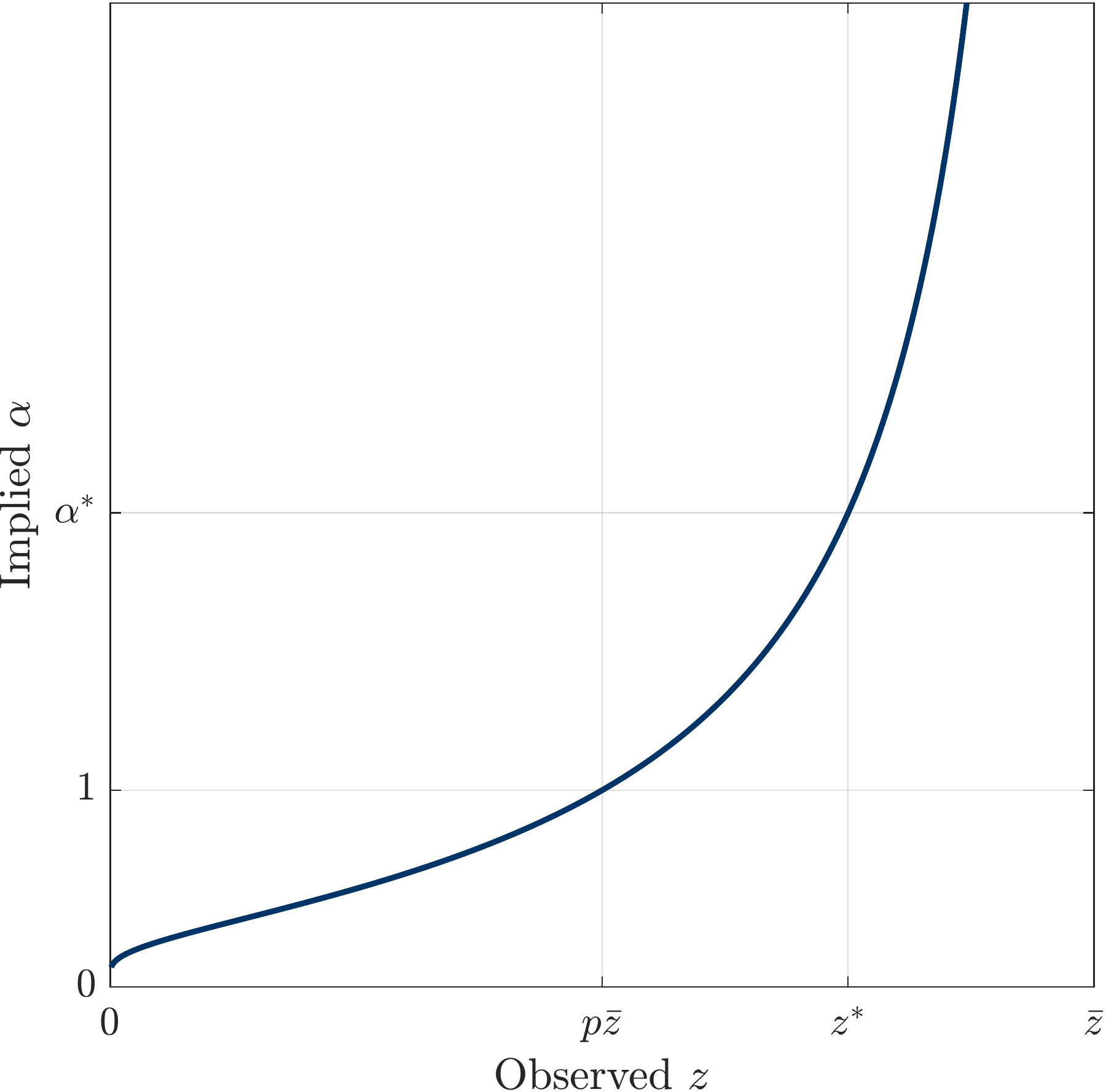
In other words, if we label this single-task experiment \(\boldsymbol Z\), then \(\Phi_{\mathcal{M}}(\boldsymbol Z|\alpha) = p^{1/\alpha}\bar z\). Because this prediction is strictly increasing in \(\alpha\), \(\Phi_{\mathcal{M}}\) is one-to-one in \(\alpha\), as illustrated in panel A of Figure 1. Hence, every realization of \(z^*\) implies a unique value of the risk-aversion parameter \(\alpha\), and therefore, \(\alpha\) is theoretically identified.
Figure 1: Identification in Example 1
Panel A: Identification with Power Utility
Panel B: Non-Identification Without \(u()\)
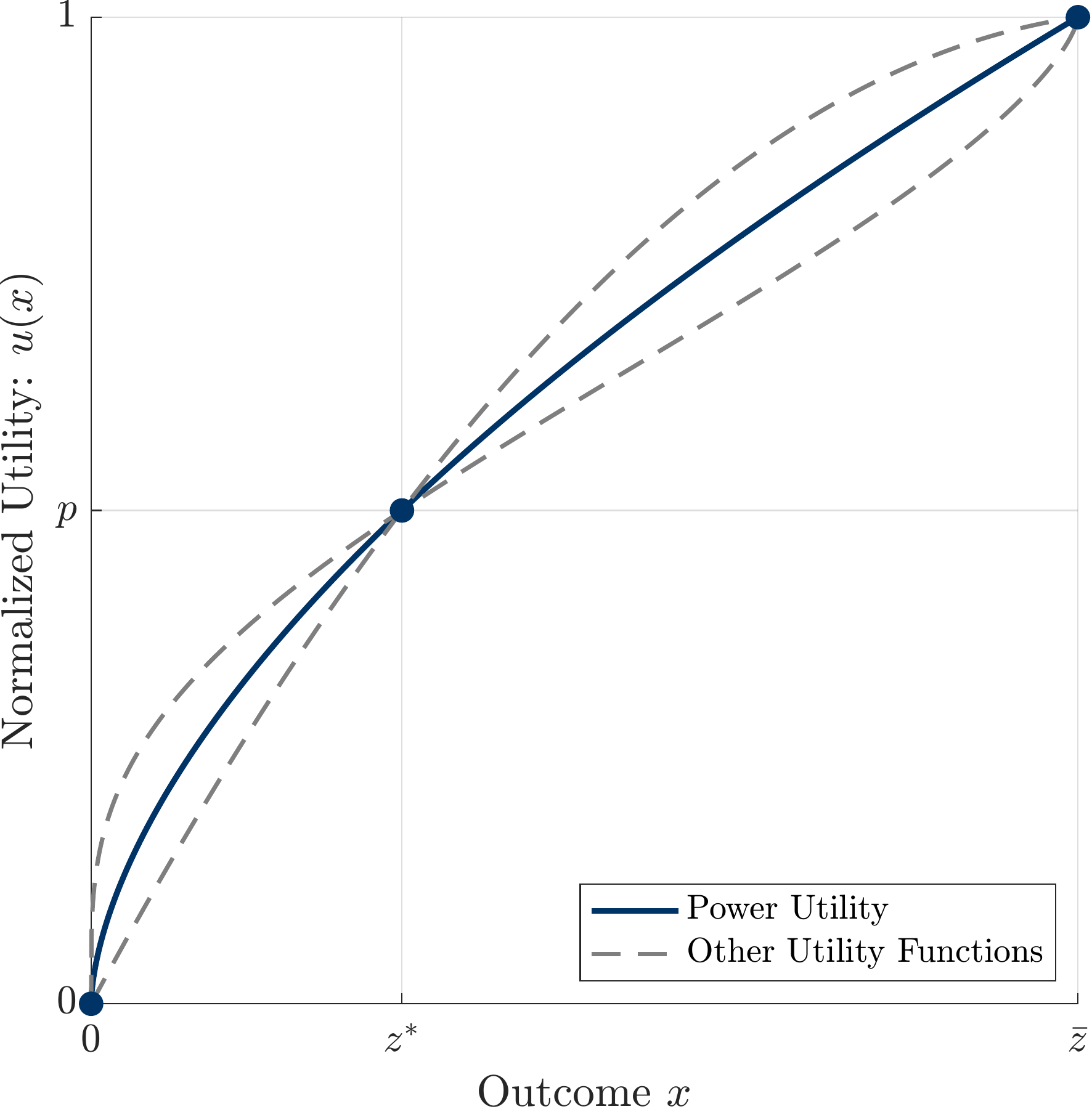
Notes: Figure illustrates identification and non-identification in Example 1, specifically from an observation that \((z^*,1) \sim (\bar z,p)\). Under the functional-form assumption of power utility \(u(x) = x^\alpha\), Panel A depicts the set of \((z,\alpha)\) combinations consistent with \((z,1) \sim (\bar z,p)\). Because each \(z\) is consistent with a unique \(\alpha\), the utility function (i.e., \(\alpha\)) is identified. For example, observing \(z = z^*\) in Panel A implies \(\alpha = \alpha^*\). In contrast, Panel B illustrates that, without any functional-form assumption on \(u(x)\), power utility is just one of many utility functions consistent with \((z^*,1) \sim (\bar z,p)\). Specifically, if we normalize the utility function such that \(u(0) = 0\) and \(u(\bar z) = 1\), then any utility function with \(u(z^*) = p\) is consistent with \((z^*,1) \sim (\bar z,p)\). Panel B illustrates three such utility functions.
Example 1 suggests a simple starting point for how to think about theoretical identification when using indifference conditions: If model \(\mathcal{M}\) has one parameter, we may be able to identify that parameter off one indifference condition, and if it has \(K\) parameters, we may be able to identify those parameters off of \(K\) indifference conditions. However, there are some important caveats to keep in mind.
First, when assessing what set of indifference conditions to use, one must make sure to use variation in probabilities or amounts that actually matter for the model under consideration. As a simple example, consider an EU model with a two-parameter utility function. Suppose that an experiment’s first valuation task is “state a \(z\) such that \((z,1) \sim (\bar z,p)\),” for which any realization would be consistent with many combinations of the two parameters of the utility function. Suppose further that the experiment’s second valuation is “state a \(z\) such that \((z,r) \sim (\bar z,pr)\).” Unfortunately, EU implies that, for any utility function, a person should provide the same valuation for both tasks. Therefore this second task would not provide the data necessary to separately identify the two parameters of the utility function.
Second, it is crucial to recognize—and be comfortable with—the extent to which identification comes from functional-form assumptions. To illustrate, consider again Example 1, but now without any functional-form assumption for \(u(x)\). If we observe an indifference condition \((z^*,1) \sim (\bar z,p)\), under EU without any functional-form assumption for \(u(x)\), the only thing we can infer about the utility function is that \(u(z^*)=pu(\bar z) + (1-p)u(0)\). Normalizing the utility function such that \(u(0)=0\) and \(u(\bar{z})=1\), we can only infer from this indifference condition that \(u(z^*)=p\).9 If we make the functional-form assumption of power utility as in Example 1, then only a single \(\alpha\) can generate a normalized utility function with \(u(0)=0\), \(u(\bar{z})=1\), and \(u(z^*)=p\). However, as illustrated in panel B, many other utility functions with different functional forms also pass through those three points.
Hence, claiming to have identified the utility function from a single indifference condition in Example 1 relies heavily on the functional-form assumption. We recommend collecting additional valuations at different locations in the lottery space to assess the importance of functional-form assumptions. Having multiple observations across the parameter space—that is, observing additional points in Figure 1b—can help us to understand how reasonable our functional-form assumptions are. Additional data also allows for more formal overidentification tests and non-parametric approaches.
While our discussion above has focused on theoretical identification using indifference conditions, similar principles apply to binary-choice data or choices from finite menus. As we saw in Section 4, behavior for each such decision restricts the set of parameters consistent with the data. The design question then becomes how to choose a set of decision tasks such that the possible realizations parse the parameter space into sufficiently fine regions.
5.1.2 Accounting for Noisy Decisions When Estimating Models of Risk Preferences
Once the researcher has established a set of questions that permit theoretical identification of the proposed model, it is essential to account for decision noise. Experimental participants frequently make different decisions when facing the same decision task within a short period (Camerer 1989; Starmer and Sugden 1989). Therefore, we cannot interpret decisions as perfect reflections of underlying preferences, and instead, we must think of decisions as noisy reflections of underlying preferences.10
We first discuss decision noise in the context of binary choices. Consider a binary choice between lotteries \(A\) and \(B\), and suppose we are considering a utility model \(\mathcal{M}\) that evaluates lotteries according to \(U(\cdot|\theta_{\mathcal{M}})\). Without noise, the model predicts that the person would choose \(A\) whenever \(U(A|\theta_{\mathcal{M}})>U(B|\theta_{\mathcal{M}})\). Decision noise means that a person might sometimes choose \(B\) even when the underlying utility model predicts they should choose \(A\).
When estimating a model, the typical way to account for decision noise is to include it formally in an expanded model. In other words, we combine an underlying model of risk preferences with a model of decision noise to generate a combined model of stochastic decision-making. The result is that, even when the underlying model predicts a deterministic choice (choose \(A\) or \(B\)), the combined model predicts stochastic choice (choose \(A\) with probability \(s\)). The exact predictions for the choice probabilities will depend on the assumptions about the noise structure.
Some early work accounted for noise by assuming that people sometimes “tremble.” Specifically, this approach assumes that there is some trembling probability \(\varepsilon\), where if the underlying utility model implies that the person prefers \(A\) over \(B\), then they will choose \(A\) with probability \(1-\varepsilon\) but will choose \(B\) with probability \(\varepsilon\) (Harless and Camerer 1994).11 However, the trembling approach has not been used much in the recent literature, largely because it does not incorporate the natural feature that whether one deviates from the option that maximizes their underlying preferences should depend on the strength of those underlying preferences.
The most common approach is to assume additive utility noise in the spirit of McFadden (1974, 1981). Hey and Orme (1994) provide an early implementation of this approach in the domain of risk preferences. The approach assumes there is some random variable \(\varepsilon_{AB}\) such that the person chooses \(A\) from choice set \(\{A,B\}\) when
\[ U(A|\theta_{\mathcal{M}})-U(B|\theta_{\mathcal{M}}) > \varepsilon_{AB}. \]
If we let \(F_{AB}(\varepsilon_{AB})\) denote the CDF for \(\varepsilon_{AB}\) with parameter \(\sigma\), the stochastic model predicts that the likelihood of choosing \(A\) from choice set \(\{A,B\}\) given utility parameters \(\theta_{\mathcal{M}}\) is
\[ \Pr(U(A|\theta_{\mathcal{M}})-U(B|\theta_{\mathcal{M}}) > \varepsilon_{AB}) = F_{AB}(U(A|\theta_{\mathcal{M}})-U(B|\theta_{\mathcal{M}})) \equiv \Pr_{\mathcal{M}}(A|\{A,B\},\theta_{\mathcal{M}},\sigma). \]
To complete this approach, we must make an assumption about the distribution of \(\varepsilon_{AB}\). Typically, researchers assume some type of symmetric mean-zero distribution where the parameter \(\sigma\) captures the spread of the distribution. The most common assumptions are that \(\varepsilon_{AB}\) has either a normal distribution with a zero mean and standard deviation \(\sigma\) or a logistic distribution with a zero mean and scale parameter \(\sigma\).12
Figure 2 illustrates the model predictions for symmetric mean-zero noise. The navy line depicts the predicted probability of choosing lottery \(A\) as a function of the utility difference between lotteries \(A\) and \(B\). With symmetric mean-zero noise, the choice probability is greater than one-half when the utility difference is positive and less than one-half when the utility difference is negative. Moreover, the choice probability approaches zero or one as the magnitude of the utility difference becomes very large. Figure 2 also illustrates how the sensitivity of the choice probability to changes in the utility difference depends on the spread of the noise distribution. The green line depicts the choice probability of choosing \(A\) when we double the scale of the error term. It shows that the sensitivity of the choice probability to changes in the utility difference is smaller as the variance gets larger. Intuitively, the larger the impact of noise, the more the choice probabilities are pulled toward 50 percent (the random choice benchmark).
Figure 2: The Impact of Noise on Choice Probabilities
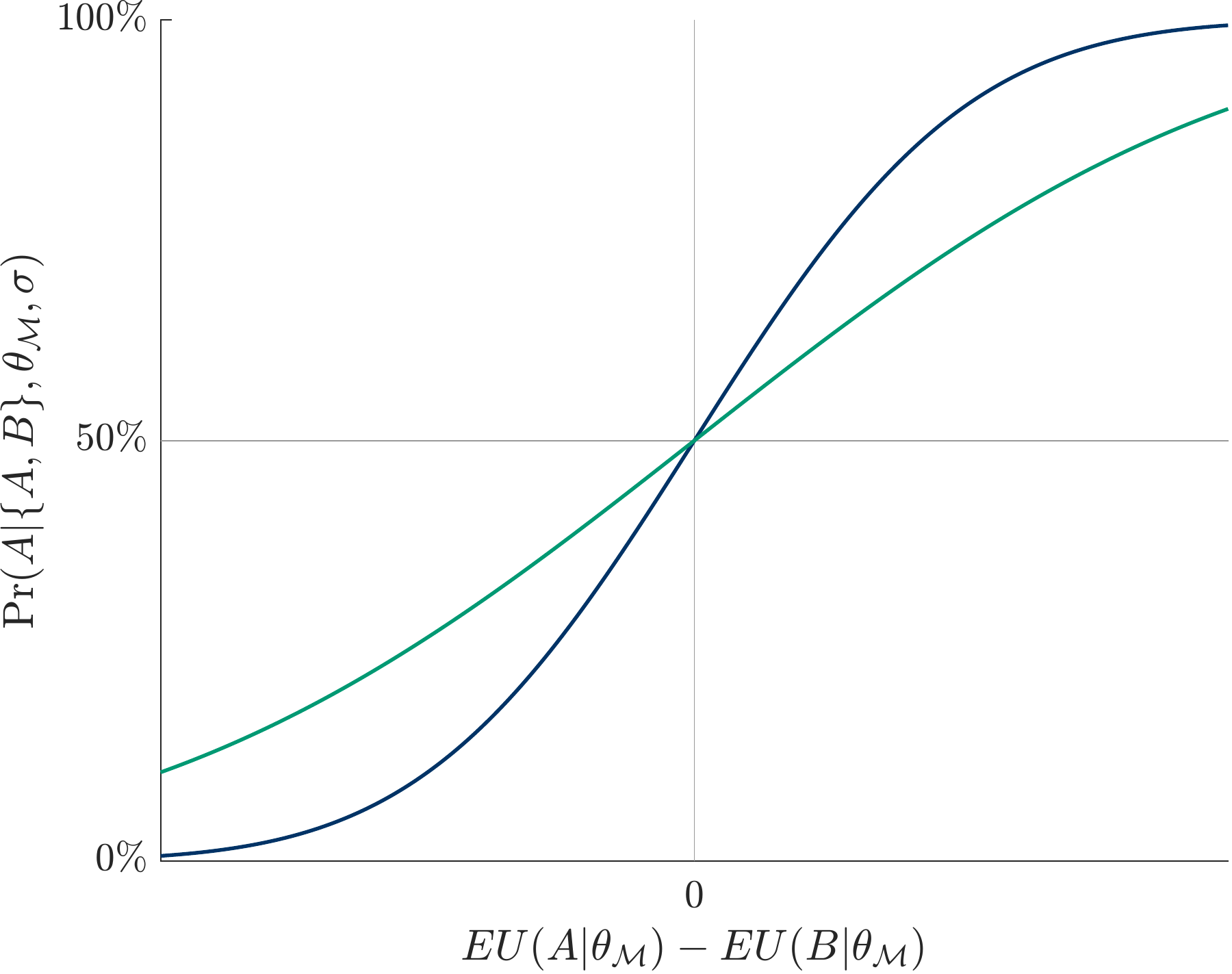
Notes: This figure illustrates the probability of choosing \(A\) from choice set \(\{A,B\}\) as a function of the expected utility difference \(EU(A|\theta_\mathcal{M}) - EU(B|\theta_\mathcal{M})\), where \(\theta_\mathcal{M}\) denotes the model parameters. The navy line depicts the case in which the error term \(\varepsilon_{AB}\) is normally distributed with mean zero and standard deviation \(\sigma\). The green line illustrates the impact of doubling the standard deviation to \(2\sigma\).
Once we have incorporated noise into the analysis, we must again think about identification. In particular, we need to consider whether we can separately identify the parameters of the underlying model of risk preferences from the parameters of the noise distribution. For binary choices, it is useful to think about identification for the ideal case where we could observe the choice shares (or choice probabilities) for each question we present to participants. Formally, consider an experiment with a series of \(N\) binary choices between \(A_n\) and \(B_n\). Suppose we observe, for each decision task \(Z_n\), the share of participants from a homogeneous participant pool that choose Option \(A_n\), which we denote by \(\psi_n\). The data will then be the vector of shares of participants choosing Option \(A_n\) across the \(N\) tasks, \(\psi = \bigl\{\psi_n \bigl\}_{n=1}^N\).
The model prediction for decision task \(Z_n\) is the predicted choice probability of choosing \(A_n\), or
\[ \Phi_{\mathcal{M}}(Z_n|\theta_{\mathcal{M}},\sigma) = \ \Pr_{\mathcal{M}}(A_n|\{A_n,B_n\},\theta_{\mathcal{M}},\sigma). \]
For an experiment \(\boldsymbol Z\) with \(N\) tasks, the model prediction is the vector of model-implied choice probabilities, \(\Phi_{\mathcal{M}}(\boldsymbol Z|\theta_{\mathcal{M}},\sigma) = \bigl\{ \Phi_{\mathcal{M}}(Z_n|\theta_{\mathcal{M}},\sigma)\bigl\}_{n=1}^N\). For identification, our goal is to design an experiment \(\boldsymbol Z\) such that, for each possible data realization \(\mathbf{\psi}\), there is a unique \((\theta_{\mathcal{M}},\sigma)\) such that \(\Phi_{\mathcal{M}}(\boldsymbol Z|\theta_{\mathcal{M}},\sigma)=\psi\).
At first glance, it is tempting to think that we can fully identify stochastic models from data on a small number of binary choice tasks. Indeed, the following example illustrates how in principle a one-parameter EU model combined with a one-parameter model of noise could be fully identified from data on two choice tasks:
Example 2: Identifying Preferences via Assumptions About Noise
Suppose model \(\mathcal{M}\) is EU with power utility \(u(x) = x^\alpha\), and let \(U(X)\) denote the EU of lottery \(X\). Suppose further that we assume additive utility noise that is the same for all choice tasks, and thus for any lotteries \(X\) and \(Y\), \(\Pr(X|\{X,Y\}) = F(U(X)-U(Y))\), where \(F\) is the CDF for the utility noise.
Suppose we present people with the following two choice tasks:
\[ \begin{array}{cccc} \text{Choice Task 1: choose between} & A \equiv (\$10,1) & vs. & B \equiv (\$25,1/2) \\ \text{Choice Task 2: choose between} & A \equiv (\$10,1) & vs. & C \equiv (\$35,1/3) \end{array} \]
Let \((s_1,s_2)\) denote the observed shares choosing \(A\) in each of the two tasks.
If we assume that the noise takes on a logistic distribution with scale parameter \(\sigma\), then
\[ F(U(X)-U(Y)) = \dfrac{1}{1+e^{-(U(X)-U(Y))/\sigma}}. \]
For many \((s_1,s_2)\) combinations that we might observe, a unique \((\alpha,\sigma)\) solves both \(F(U(A)-U(B))=s_1\) and \(F(U(A)-U(C))=s_2\). For instance, panel A in Figure 3 depicts the set of \((\alpha,\sigma)\) combinations consistent with \(s_1=0.7\) (navy curve) and \(s_2=0.9\) (green curve). As these curves intersect at a unique point, from this pair of binary choices we would conclude that \((\alpha^*_1,\sigma^*_1)=(0.645,0.507)\).
But if we instead assume that the noise takes on a uniform distribution on support \([-\sigma,\sigma]\), then
\[ F(U(X)-U(Y)) = \frac{(U(X)-U(Y))-(-\sigma)}{2\sigma}. \]
Again, for many \((s_1,s_2)\) combinations that we might observe, a unique \((\alpha,\sigma)\) solves both \(F(U(A)-U(B))=s_1\) and \(F(U(A)-U(C))=s_2\). For instance, panel B in Figure 3 depicts the set of \((\alpha,\sigma)\) combinations consistent with \(s_1=0.7\) (dashed navy curve) and \(s_2=0.9\) (dashed green curve), and we would conclude that \((\alpha^*_2,\sigma^*_2)=(0.563,1.486)\).
Hence, under either assumption about the noise distribution, we can identify both the parameter of interest \(\alpha\) and the magnitude of the noise; however, the different assumptions about the noise distribution can lead to different estimates for \(\alpha\).13
Figure 3: Identification of \((\alpha,\sigma)\) from Two Choice Probabilities
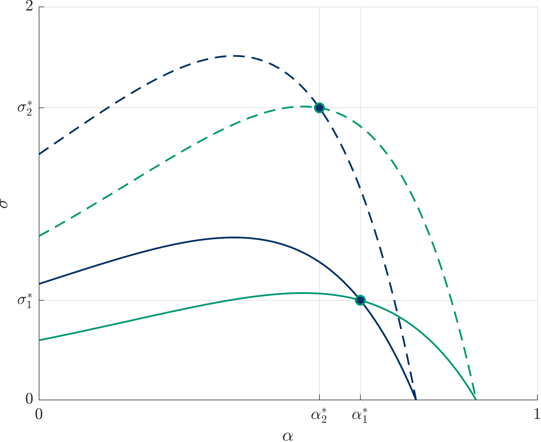
Notes: This figure illustrates the importance of noise in identifying the risk-preference parameter \(\alpha\) as described in Example 2. This example supposes we observe the choice shares for the choice task \(A \equiv (\$10,1)\) vs. \(B \equiv (\$25,1/2)\) and for the choice task \(A \equiv (\$10,1)\) vs. \(C \equiv (\$35,1/3)\). The share choosing \(A\) is 70 percent in the first choice and 90 percent in the second. The navy lines depict the set of \((\alpha,\sigma)\) combinations consistent with the first choice share, and the green lines depict the \((\alpha,\sigma)\) combinations with the second. The solid lines depict the case of logistic noise with scale parameter \(\sigma\), and the dashed lines depict uniform noise with support \([-\sigma,\sigma]\). The two intersection points denote the unique combination consistent with both.
Example 2 is a cautionary one: In principle, we can identify both the preference and the noise parameters from data on two choice tasks, but this conclusion relies on functional-form assumptions for both the utility function and noise. Moreover, we highlight that the identification also depends on the assumption that the distribution of the choice noise is the same for both choice tasks; that is, we have assumed the same \(\sigma\) applies to all individuals for both choice tasks. While this latter assumption might seem innocuous, we highlight later reasons why it might not be.
Recall from Section 5.1 that two binary choice tasks only allow us to partition the \(\alpha\) parameter space into relatively coarse bins in the absence of decision noise. If we instead think that people’s choices are noisy reflections of their underlying preferences, identifying those preferences should be more data-intensive, not less. The fact that the identification becomes easier in Example 2 highlights just how strong an assumption it is to assume that we know the noise structure. In practice, we encourage researchers to embrace our point from Section 5.1.1: the first design step is to ensure theoretical identification by making sure that one has a set of binary choices that would sufficiently identify the model of risk preferences in a world where choices perfectly reflect underlying preferences. When assessing how to account for noise, one should expect to need additional questions, not fewer.
In addition to ensuring the identification of the stochastic model, we need to devise a strategy for the actual estimation when accounting for noise. The discussion above describes parameter estimation in terms of comparing choice shares in the data with those predicted by the stochastic model. In practice, this suggests using a procedure akin to generalized method of moments to estimate parameters.
However, the more common approach is to use maximum likelihood. To illustrate this approach, we return to thinking of a data realization as a vector of chosen options \(\mathbf{\psi} \equiv (\psi_1,...,\psi_N)\) from a vector of binary choice tasks \(\boldsymbol Z \equiv (Z_1,...,Z_N)\).14 From above, the model-implied probability that we observe any particular choice \(\psi_n\) from \(Z_n\) is \(\Pr_{\mathcal{M}}(\psi_n|Z_n,\theta_{\mathcal{M}},\sigma)\). We can then construct the log-likelihood of observing data \(\mathbf{\psi}\) given parameters \((\theta_{\mathcal{M}},\sigma)\):
\[ \mathcal{L}(\mathbf{\psi}|\boldsymbol Z,\theta_{\mathcal{M}},\sigma) \equiv \sum_{n=1}^N log \left( \Pr_{\mathcal{M}}(\psi_n|Z_n,\theta_{\mathcal{M}},\sigma) \right). \tag{1} \]
Much of the discussion above may look familiar from what the reader has seen in other domains. However, there is one important dimension that applies under risk that doesn’t typically arise in some other domains. Specifically, in some domains, such as estimating utilities for options in structural IO, utility does not have a natural scale, and thus, we cannot separately identify the scale of utility and the scale of noise. A common approach in such situations is to normalize the scale of noise; for example, to assume a logistic distribution with \(\sigma=1\). In contrast, models of risk preferences frequently come to us with the scale already normalized. In such situations, one must include the scale of the noise as one of the objects to be estimated.
It is straightforward to apply the estimation approach above to data from MPL valuations. Recall that an MPL is an ordered sequence of choices. As such, it is possible to apply the approach above directly by treating each choice in the MPL as an independent observation with an independent noise draw. However, the assumption of independent noise draws for each choice in an MPL seems somewhat unreasonable, especially if one takes the common approach of ignoring multiple switching within a list—a feature that would naturally arise with independent error draws.
A more reasonable approach is to treat the choices within an MPL as correlated, and indeed, recent work often treats an MPL as being driven by a single noise draw applied to all rows.15 With this assumption, we can construct a modified log-likelihood function. To illustrate, consider an MPL where Option \(A\) is fixed across rows while Option \(B(y)\) varies via a dollar outcome \(y\) that increases across rows in \(\$1\) increments. Data for this MPL comes in the form of the maximum \(y\) in the list such that the person chooses \(A\) over \(B(y)\). In other words, a data realization \(\psi_n\) for an MPL decision task \(Z_n\) is such that the participant chooses \(A\) over \(B(\psi_n)\) but \(B(\psi_n + \$1)\) over \(A\). Hence, if we assume a single noise draw \(\varepsilon\) with CDF \(F(\varepsilon)\), the model-predicted probability of observing data realization \(\psi_n\) is
\[ \begin{array}{ccl} \Pr_{\mathcal{M}}(\psi|Z_n,\theta_{\mathcal{M}},\sigma) & = & \Pr(U(A|\theta_{\mathcal{M}})-U(B(\psi_n)|\theta_{\mathcal{M}}) > \varepsilon > U(A|\theta_{\mathcal{M}})-U(B(\psi_n+\$1)|\theta_{\mathcal{M}})) \\ & = & F(U(A|\theta_{\mathcal{M}})-U(B(\psi_n)|\theta_{\mathcal{M}})) - F(U(A|\theta_{\mathcal{M}})-U(B(\psi_n+\$1)|\theta_{\mathcal{M}})). \end{array} \]
We can then use \(\Pr_{\mathcal{M}}(\psi_n|Z_n,\theta_{\mathcal{M}},\sigma)\) for data on multiple MPLs to construct a log-likelihood function as in equation (1).
Another benefit of gathering valuation data is its suitability for minimum-distance estimation. To use this method, we must convert switching rows into a specific indifference value. Typically, researchers calculate the average values between the two switching rows as the indifference point. For example, if we observe that a participant chooses \(A\) over \(B(\psi_n)\) but \(B(\psi_n + \$1)\) over \(A\), we would take the indifference value as \(\psi_n+\$0.50\). This method involves a loss of information, so the decision to use it should depend on how large the increments in the MPL are.
The data are now in the form of a vector of indifference values \(\mathbf{\psi} \equiv (\psi_1,...,\psi_N)\), and the underlying model \(\mathcal{M}\) generates model-predicted indifference values \(\mathbf{\psi}^*(\theta_{\mathcal{M}}) \equiv (\psi^*_1(\theta_{\mathcal{M}}),...,\psi^*_N(\theta_{\mathcal{M}}))\). We can then use some form of minimum-distance estimation to estimate the \(\theta_{\mathcal{M}}\) that minimizes the distance between the data and the fitted model. For example, we can use non-linear least squares to estimate,
\[ \psi_n = \psi^*_n(\theta_{\mathcal{M}}) + \epsilon_n, \]
where \(\epsilon_n\) is an error term. A major advantage of a minimum-distance approach is that it does not require any assumptions about the distribution of noise.
Before moving on, we briefly discuss two design strategies to collect data that can better account for noise. First, collecting repeat observations for the same individual on the same decision task can be helpful. If the response for each decision task is influenced both by preferences and by noise, and the preference component is constant while the noise components are independent, then we obtain some ability to separate the preference from the noise. To implement this approach, we recommend putting some temporal and task distance between the multiple instances of the same decision task to make it more plausible that there are separate, independent noise draws.
Second, we can directly test our assumptions about the noise structure by investigating whether the distribution of the data is consistent with that structure. For example, we can use our estimates to calculate the predicted distribution of behavior, and then compare that predicted distribution to the actual distribution of behavior in the data. Substantial differences between the actual and fitted values would suggest that the error structure may be misspecified.
5.1.3 Accounting for Heterogeneity When Estimating Parameters
Individuals differ substantially in their appetite for or aversion to risk, as evident from the rich array of customizable insurance policies and the ability to bet on a seemingly endless combination of outcomes on sports betting websites. Hence, when estimating models of risk preferences, it is essential to account for individual heterogeneity.
The most direct way to account for heterogeneity is to eliminate it by estimating the model of risk preferences separately for each participant. This approach means that we obtain an individual-specific estimate \(\theta_{\mathcal{M},i}\) for each individual \(i\). Of course, this approach requires a design where we collect sufficient data from each individual. While it is sometimes possible to implement many decisions in experimental settings, in practice, researchers usually avoid overburdening respondents with too many questions.
Alternatively, we can build heterogeneity into the model by positing a population distribution for \(\theta_{\mathcal{M}}\). Perhaps the simplest version is to estimate a finite mixture model in which we assume there is some finite number \(K\) of types, where each type \(k\) is permitted to have their own \(\theta_{\mathcal{M},k}\). We then let \(\gamma_k\) be the proportion of the population that is type \(k\), which means we need to estimate the vector \(\Gamma \equiv (\gamma_1,...,\gamma_K)\). In a maximum-likelihood estimation (MLE) approach, we can build on the likelihood function in equation (1) in the prior section to derive the new likelihood function: If we present an individual with a set of choice tasks \(\boldsymbol Z\) and their behavior is captured by the vector \(\mathbf{\psi}\), the log-likelihood for that individual is
\[ \mathcal{L}^*(\mathbf{\psi}|\boldsymbol Z,\theta_{\mathcal{M}},\sigma,\Gamma) \equiv \sum_{k=1}^K \gamma_k \mathcal{L}(\psi|\boldsymbol Z,\theta_{\mathcal{M},k},\sigma). \]
We then sum the individual log-likelihoods to get the sample log-likelihood. Bruhin et al. (2010) apply this approach when estimating CPT from experimental data. In principle, we can estimate the model for different values of \(K\), and then use some statistical criterion to select the best \(K\). However, likelihood functions for finite mixture models can become quite flat once there are more than a few types, leading to major computational problems and reducing confidence in identification.
Instead of a finite mixture model, one can reduce the dimensionality of the problem by assuming a parameterized population distribution for \(\theta_{\mathcal{M}}\). For instance, for EU with CRRA, one might assume that \(\alpha \sim N(\bar \alpha,\sigma_\alpha^2)\) and thus have just two \(\theta_{\mathcal{M}}\) parameters to estimate.16 More generally, if \(G(\theta)\) is the CDF for \(\theta_{\mathcal{M}}\), the log-likelihood for an individual is
\[ \mathcal{L}^*(\mathbf{\psi}|\boldsymbol Z,\theta_{\mathcal{M}},\sigma,\Gamma) \equiv \int_G \mathcal{L}(\psi|\boldsymbol Z,\theta,\sigma)dG(\theta). \]
To make the estimation computationally feasible, the standard approach is to use simulated maximum likelihood estimation (Train 2009).
There is an important potential pitfall to keep in mind when one permits heterogeneous risk preferences: be careful not to assume homogeneous noise. The reason relates again to the fact that most models of risk preferences come to us with the scale already normalized. The crucial additional point is that most models also have the feature that the scale varies with the model’s parameters in a way that does not relate to the strength of preferences. To illustrate, consider the following example:
Example 3: Heterogeneous Preferences and Homogeneous Noise
Consider persons 1 and 2, whose risk preferences both take the form of EU with power utility. Person 1 has \(\alpha_1 = 1/2\) while person 2 has \(\alpha_2 = 1/4\), and therefore person 2 is more risk averse than person 1. Suppose we present both people with the binary choice:
\[ A \equiv (\$16,1) \qquad \textbf{ versus } \qquad B \equiv (\$81,1/4). \]
In terms of their underlying preferences, both prefer lottery \(A\), but the more risk-averse person 2 has a stronger preference in the sense that their certainty equivalent for lottery \(B\) ($0.32) is smaller than that for person 1 ($5.06). However, the utility differences are:
\[ \begin{array}{ll} EU_1(A) - EU_1(B) = (16)^{0.5} - 0.25(81)^{0.5} & = 1.75, \quad \text{ and } \\ EU_2(A) - EU_2(B) = (16)^{0.25} -0.25(81)^{0.25} & = 1.25. \end{array} \]
Even though person 2 has a stronger preference for \(A\) over \(B\), their utility difference is smaller. Hence, if we were to assume additive utility noise that is homogeneous across the two people, person 2 would be more influenced by the noise—in particular, with homogeneous mean-zero noise, person 2 would be more likely to choose lottery \(B\) than person 1 would be.
Example 3 is again cautionary: when permitting heterogeneous risk preferences, it is also best practice to allow heterogeneous noise. With the typical specifications for power utility, CRRA utility, and CARA utility described in Section 3.1, for any two lotteries \(X\) and \(Y\), the magnitude \(|EU(X)-EU(Y)|\) declines toward zero as the preference parameter goes in the direction of making the person more risk averse.17 If so, then homogeneous noise will have a larger impact on people who are more risk averse. While this might turn out to be empirically accurate ex-post, it is not something we ought to impose ex-ante via the structure of the model. Rather, it is something that we should conclude from data by permitting heterogeneous noise and estimating how noise varies with preference parameters.18
Recognizing these issues, it is important to account for heterogeneity at the design stage. Perhaps most importantly, one must collect multiple observations from each individual. From a pure cross-section, it is impossible to separately identify heterogeneity in preferences from decision noise unless one makes strong assumptions about distributions. Indeed, the more observations we have for each individual, the more able we can distinguish the two; intuitively, we get closer to the world where we can estimate the model separately for each individual. Finally, we reiterate our point from Section 5.1.2 that collecting repeat observations from the same individual on the same decision task can be valuable. This data provides the ideal variation for identifying heterogeneity in pure noise at the individual level: When an individual makes the same decision many times, deviations are solely due to noise. The consistency of behavior across these decisions thus provides a measure of noise and permits stronger identification of a model with heterogeneous noise.
5.2 Design and Analysis When Testing Properties
In this section, we describe how to think about the issues of theoretical identification, decision noise, and heterogeneity in the context of testing properties of risk preferences. Throughout, we emphasize two main themes. First, regardless of the type of data one plans to collect, reframing properties in terms of underlying indifference values can be useful. Second, in the context of testing properties, valuation tasks can have some important advantages relative to binary choice tasks. Here, we illustrate those advantages assuming that binary choice tasks and valuation tasks both yield unbiased measures of one’s underlying preferences. In Section 6.2, we discuss the issue of whether either might yield biased measures.
5.2.1 Identification When Testing Properties
For research focused on testing properties of risk preferences, the analog of ensuring theoretical identification is ensuring that we turn a precisely specified property into a precisely specified empirical test under the assumption that decisions solely reflect underlying risk preferences.
The properties of risk preferences described in Section 3.2 are all expressed in terms of conditions on a binary preference relation. If we assume that risk preferences are continuous and monotonically increasing in amounts, we can convert those conditions into properties expressed in terms of underlying indifference values. To illustrate, consider first the simple property of global risk aversion, which states that, for any non-degenerate lottery \(X\), \((E(X),1) \succ X\). Converting this property into a condition on indifference values is straightforward. For any lottery \(X\), continuity and monotonicity imply that the person’s preferences involve a unique value \(y^*\) such that \((y^*,1) \sim X\). The property of global risk aversion then becomes \(y^* < E(X)\). This property is easy to translate into precise empirical tests. For instance, if we want to use binary choice tasks, we can present participants with binary choices where each involves choosing between non-degenerate lotteries versus getting the expected value of that lottery for sure and test whether people choose the latter. Alternatively, for valuation tasks, we can elicit certainty equivalents for lotteries and test whether the certainty equivalent is smaller than the expected value of the lottery.
Many properties, such as the independence axiom or the directional alternatives of the CRE or CCE, state that one condition implies another. Tests of such properties require comparing behavior across pairs of decision tasks. For instance, to test the null of the independence axiom, we can present participants with two decision tasks in which the second is created from the first via a transformation that should not alter behavior according to the independence axiom.
As an example, consider common ratio manipulations that test the null of the independence axiom against the alternative of the CRE. For experimental parameters \((m,h,p,r)\) with \(h>m>0\) and \(p,r \in (0,1)\), the independence-axiom null is that \((h,p) \succsim (m,1)\) if and only if \((h,pr) \succsim (m,r)\), and the CRE alternative is that \((h,p) \succsim (m,1)\) implies \((h,pr) \succ (m,r)\). Historically, researchers have conducted such tests using the following CR paired choice task:19
\[ \begin{array}{lll} \text{\textbf{$\boldsymbol{A B}$ Choice Task}}\text{:\quad choose Lottery }A \equiv (m,1)\qquad &\text{versus\quad Lottery }B\equiv (h,p) \\ \text{\textbf{$\boldsymbol{C D}$ Choice Task}}\text{:\quad choose Lottery }C \equiv (m,r)\qquad &\text{versus\quad Lottery }D\equiv (h,pr) \end{array} \]
For this paired choice task, choosing \(A\) and \(C\) or \(B\) and \(D\) are both consistent with the independence axiom, whereas choosing \(A\) and \(D\) is inconsistent with the independence axiom and consistent with the CRE alternative.
Now, consider how converting the independence axiom and the CRE properties into conditions on indifference values can be useful. There are several ways to achieve this. For instance, if we fix the experimental parameters \((h,p,r)\), continuity and monotonicity imply that the person’s preferences involve unique values \((m^*_{AB},m^*_{CD})\) such that \((m^*_{AB},1) \sim (h,p)\) and \((m^*_{CD},r) \sim (h,pr)\). The null of the independence axiom then becomes \(m^*_{AB}=m^*_{CD}\), and the CRE alternative becomes \(m^*_{AB}<m^*_{CD}\).
This structure can provide valuable guidance for designing an effective CR paired choice task. Recall that observing the choice combination \(A\) and \(D\) is inconsistent with the independence axiom and consistent with the CRE. However, the CRE prediction is not that a participant should choose \(A\) and \(D\) for any CR paired choice task. Rather, for a fixed \((h,p,r)\), the prediction is that we should observe \(A\) and \(D\) only if the experimenter chooses the value of \(m\) such that \(m^*_{AB}<m<m^*_{CD}\). If we select an \(m\) that is too large (i.e., \(m>m^*_{CD}\)), the participant will choose combination \(A\) and \(C\), and if we choose \(m\) too small (i.e., \(m<m^*_{AB}\)), the participant will choose combination \(B\) and \(D\). Hence, designing an effective CR paired choice task requires careful selection of the experimental parameters (\(m\) in this example) to ensure that the participant’s choices will reveal their underlying CRE.
McGranaghan et al. (2024) highlight how one can remove the need for such artful design by instead using the following CR paired valuation task:
\[ \begin{array}{llll} \text{\textbf{$\boldsymbol{A B}$ Valuation Task}}\text{:\quad state an $m_{AB}$ \hspace{1pt}such that} & (m_{AB},1) & \sim & (h,p) \\ \text{\textbf{$\boldsymbol{C D}$ Valuation Task}}\text{:\quad state an $m_{CD}$ such that} & (m_{CD},r) & \sim & (h,pr). \end{array} \]
A CR paired valuation task maps directly to our structure of underlying indifference values. Hence, for any experimental parameters \((h,p,r)\), we can test the null of the independence axiom by testing whether \(m_{AB}=m_{CD}\), and we can look for evidence consistent with the CRE by seeing whether \(m_{AB} < m_{CD}\). Intuitively, conducting a paired valuation task is akin to conducting many paired choice tasks for different values of \(m\), and thus, it is likely that one of them will be in the participant’s sweet spot. Beyond eliminating the need for artful design, a second advantage of CR paired valuation tasks is that they provide a measure of the magnitude of the effect via the measure \(m_{CD}-m_{AB}\). In contrast, a CR paired choice task can only reveal whether a person has a CRE.
Another aspect of ensuring theoretical identification when testing properties of risk preferences is to make sure the test reflects the domain of the property. For instance, if the proposed property is global risk aversion, we cannot merely test for risk aversion on a small number of gambles. Instead, we must test for risk aversion across a broad set of different lotteries. Similarly, if the proposed property is a global CRE, we must test for a CRE for a broad range of experimental parameters \((h,m,p,r)\). Unfortunately, this has not always been the case in the prior literature. McGranaghan et al. (2026) highlight how the prior experimental literature on both the CRE and the CCE has focused on a relatively narrow range of experimental parameters dominated by the influence of canonical parameters in Allais (1953) and Kahneman and Tversky (1979).
5.2.2 Accounting for Noisy Decisions When Testing Properties
Even when a precise test is available for a theoretically identified property, it is critical to assess whether decision noise might compromise that test. In fact, decision noise can create severe problems for tests that involve comparing behavior across binary choice tasks. To illustrate, we return to our example of CR paired choice tasks.20 As discussed in Section 5.1.2, decision noise predicts probabilistic behavior in binary choice tasks. Assuming homogeneous preferences for the moment, one might think we can simply test the null of \(\Pr(A|\{A,B\}) = \Pr(C|\{C,D\})\) against the alternative of \(\Pr(A|\{A,B\}) > \Pr(C|\{C,D\})\). Example 4 illustrates that this conjecture is incorrect.
Example 4: CRE in Binary Choices Despite Satisfying Independence
Suppose that a person’s risk preferences satisfy the independence axiom and that they prefer Options \(A\) and \(C\) in a CR paired choice task. However, decision noise also impacts their choices such that their actual choice probabilities satisfy \(1>\Pr(A|\{A,B\})>1/2\) and \(1>\Pr(C|\{C,D\})>1/2\). If the noise is more impactful for the \(CD\) task and thus pushes that choice probability closer to 50 percent, the person will have \(\Pr(A|\{A ,B\}) > \Pr(C|\{C,D\}) > 1/2\). In other words, the person would exhibit a CRE despite their underlying risk preferences satisfying the independence axiom.
Extrapolating from Example 4, testing the independence axiom by testing the null of \(\Pr(A|\{A ,B\})\) \(=\) \(\Pr(C|\{C,D\})\) is valid only under the knife-edge case where the decision noise has the same impact for both choice tasks. In fact, there are natural reasons to think this assumption is unlikely to hold. Several papers have pointed out that the common assumption of EU with additive i.i.d. utility noise will generate a CRE whenever one chooses experimental parameters such that a participant’s underlying preferences favor \(A\) and \(C\) (Ballinger and Wilcox 1997; Loomes 2005; Hey 2005; Wilcox 2008; Blavatskyy 2007, 2010; Bhatia and Loomes 2017). The key intuition is that when we scale down the probabilities by a common ratio, we also scale down the utility differences by the same common ratio, and thus the i.i.d. decision noise is more impactful for the \(CD\) choice task. McGranaghan et al. (2024) builds on this intuition and argues that the problem is not unique to the CRE property. Any test based on comparing multiple binary choice tasks will be problematic unless there is a strong reason to believe that decision noise will be equally impactful for each binary choice task.
An early solution to the issue of decision noise was to explicitly model it using parametric assumptions and develop a corresponding test statistic for the property under consideration. For example, Conlisk (1989) developed a test of the independence-axiom null based on the assumption that all deviations from that null are due to random trembling. However, a major drawback of this approach is that the test becomes a joint test of the property of risk preferences and the error structure. More recently, McGranaghan et al. (2024) argue that a more straightforward solution is to use the paired valuation tasks described in Section 5.2.1. For example, for a CR paired valuation task, if with decision noise \(m_{AB}\) and \(m_{CD}\) are still unbiased measures of the underlying indifference values \(m^*_{AB}\) and \(m^*_{CD}\), then we can test the independence axiom by testing the null of \(m_{AB}=m_{CD}\), and a finding of \(m_{AB}<m_{CD}\) is evidence of the CRE.21
If one is willing to make functional-form assumptions about decision noise, another approach to accounting for noise when using binary choice data is to collect data on multiple similar choices to estimate the underlying indifference values along with the noise distribution. For example, suppose we present participants with multiple CR paired choice tasks with the same \((h,p,r)\) but which differ in \(m\). If we assume homogeneous preferences, then everyone’s underlying indifference values are some \((m^*_{AB},m^*_{CD})\), and our goal is to estimate these.22 In terms of the decision noise, one approach is to assume that the person chooses according to effective indifference values \(m_{AB}=m^*_{AB}+\varepsilon_{AB}\) and \(m_{CD}=m^*_{CD}+\varepsilon_{CD}\). In other words, in the \(AB\) choice task, the person chooses \(A\) if \(m > m_{AB}\) and \(B\) if \(m < m_{AB}\), and the person chooses analogously in the \(CD\) choice task. Finally, if we assume that \(\varepsilon_{AB}\) and \(\varepsilon_{CD}\) have independent mean-zero normal distributions with variances \(\sigma^2_{AB}\) and \(\sigma^2_{CD}\), then the effective indifference values have a joint normal distribution.
Given this structure, if one has data from a homogeneous population on behavior for multiple CR paired choice tasks that all have the same \((h,p,r)\) but which differ in \(m\), it is straightforward to derive the model-implied choice probability for any observation. For instance, if we observe that a person was presented with a CR paired choice task with \(m=m_0\) and chose combination \(A\) and \(D\), the model-implied choice probability is \(\Pr(m_0>m_{AB} \cap m_0 < m_{CD})\). Hence, we can construct a log-likelihood function and estimate the parameters.
While this approach is feasible, we note two points. First, this approach relies heavily on the assumed functional form of noise. In contrast, the test based on CR paired valuation data only needs an assumption that the noise is additive and mean-zero. Second, identification under this approach requires, for fixed values of \((h,p,r)\), observing choice shares in CR paired choice tasks for multiple values of \(m\). As such, pursuing this approach is already moving in the direction of conducting a CR valuation task for that same \((h,p,r)\), except that under an assumption of homogeneous preferences, we could use this approach using data in which each participant completes only one CR paired choice task.
5.2.3 Accounting for Heterogeneity When Testing Properties
Much as for research on estimating models of risk preferences, heterogeneity can lead to biased inference when testing properties. Again, we emphasize the importance of thinking carefully about both heterogeneity in risk preferences and heterogeneity in the impact of decision noise. To illustrate the potential pitfalls of failing to account for heterogeneity, consider the following example:
Example 5: Heterogeneity, Noise, and a CRE in Binary Choices under Independence
Suppose all individuals satisfy the independence axiom; thus, no one has a CRE. However, there is heterogeneity in risk preferences such that, when presented with one particular CR paired choice task, 2/3 of the population prefer \(A\) and \(C\), while 1/3 of the population prefer \(B\) and \(D\).
In addition, there is heterogeneity in the impact of decision noise. Specifically, noise does not impact the latter group at all, and therefore they all choose \(B\) and \(D\). In contrast, noise does not impact the \(AB\) choice of the former group, but it substantially impacts their \(CD\) choice such that they choose approximately randomly. As a result, half of this group chooses \(A\) and \(C\), while the other half chooses \(A\) and \(D\).
Aggregating the choice shares across all participants, we would observe \(\Pr(A|\{A,B\})=2/3\) while \(\Pr(C|\{C,D\})=1/3\). In other words, the data appear to indicate substantial CRE among participants despite none having a CRE.23
While we described Example 5 in the context of the CRE, nothing in the example relies on particular features of that environment. In other words, we could have set the example in the context of any pair of binary choice tasks. Moreover, while the outcome in Example 5 does rely on some extreme assumptions about the heterogeneity in the impact of noise, the more general point is that different combinations of heterogeneity in preferences and the impact of noise can generate a variety of apparent patterns in data from paired choice tasks that may not accurately reflect underlying preferences.
Much as for dealing with decision noise, using paired valuations in place of paired binary choices can be a means to achieve valid inference when there is heterogeneity in risk preferences and the impact of noise.24 To illustrate, consider a CR problem with a fixed \((h,p,r)\), for which each individual’s underlying preferences are characterized by their \(m^*_{CD,i}-m^*_{AB,i}\). Recognizing this preference heterogeneity, our interest is in the distribution of this object—for example, we might want to assess what share of participants have a CRE, what share exhibits a reverse CRE, and what share is consistent with the independence axiom. If we present participants with a CR paired valuation task, each individual’s \(m_{CD,i}-m_{AB,i}\) is a noisy measure of their underlying preference, and under relatively weak assumptions it can be an unbiased measure. If so, taking a population average of \(m_{CD,i}-m_{AB,i}\) leads to an unbiased aggregate test.
A final advantage of using valuations is that repeat observations of the same valuations allow the experimenter to isolate the impact of noise and get a more precise measure of the distribution of underlying preferences. Specifically, we can decompose participants’ observed \(m_{CD,i}-m_{AB,i}\) into the part due to their underlying preferences \(m^*_{CD,i}-m^*_{AB,i}\) and the part due to noise.25 To illustrate, suppose that we elicit each valuation twice for each participant, where we label the four valuations \(m_{AB,i}^1\), \(m_{AB,i}^2\), \(m_{CD,i}^1\), and \(m_{CD,i}^2\). In addition, suppose that these valuations satisfy, \(m^k_{AB,i} = m^*_{AB,i} + \varepsilon^k_{AB}\) and \(m^k_{CD,i} = m^*_{CD,i} + \varepsilon^k_{CD}\) for \(k \in \{1,2\}\), where the \(\varepsilon^k_{AB}\) and \(\varepsilon^k_{CD}\) terms are independent of each other and the underlying preferences. In other words, a participant’s underlying preferences are constant across the two elicitations but are subject to two independent noise draws.
Under these assumptions, the sample covariance between \(m^1_{AB,i}\) and \(m^2_{AB,i}\) is a measure of the variance of \(m^*_{AB,i}\), while the sample covariance between \(m^1_{CD,i}\) and \(m^2_{CD,i}\) is a measure of the variance of \(m^*_{CD,i}\). Intuitively, the strength of the correlation across repeat observations provides a measure of the extent to which such measures are driven by underlying preferences. Furthermore, we can combine these terms with the sample covariance between \(m^k_{AB,i}\) and \(m^k_{CD,i}\) to obtain a measure of the covariance between \(m^*_{AB,i}\) and \(m^*_{CD,i}\), from which we can also obtain a measure of the variance of the underlying preferences \(m^*_{AB,i}-m^*_{CD,i}\).
6 Methodological and Implementation Considerations
6.1 Power Analysis
When designing any experiment, power analysis can help determine an appropriate sample size and the size of the effect the study can detect. A common approach is for the researcher to decide what the minimum effect size would need to be for a finding to be economically meaningful and then target a sample size that delivers sufficient power (typically 80%) while limiting the likelihood of a false positive (typically 5%).
This exercise is straightforward for standard treatment-control designs in which the experimenter compares one or more discrete interventions to a baseline group. As noted in Section 5, however, experiments that investigate risk aversion typically do not take a simple treatment-control format. Instead, such experiments frequently have rich variation in probabilities or outcomes and perhaps even in the number of lotteries under consideration. This variation is instrumental in identifying parameters or properties of risk preferences, but it complicates the power analysis.
For such experiments, an effective approach to power analysis is to implement Monte Carlo simulations to generate hypothetical experimental data under different assumptions about how participants respond to the decision task. For example, one might assume that CPT plus an additive i.i.d. noise term is the true underlying model governing responses in binary choice tasks, and simulate the choices of \(N\) hypothetical participants that go through the proposed design. We can then use this simulated data to estimate the proposed model or test model properties. By varying assumptions about the noise structure, underlying model, and parameter magnitudes, one can assess both the type I (false positives) and type II (false negatives) error rates.
An additional benefit of this approach is that it forces the researcher to think carefully about their analysis ex-ante. It also serves as a validation check on identification by allowing the researcher to assess whether the true underlying parameters of the model used to generate simulated data can be recovered with the proposed experimental variation. However, it is important to bear in mind that this approach also requires making strong assumptions about the data-generating process, which can lead to overly precise power conclusions that might not be valid if participant behavior deviates from the specified model. Therefore, we encourage a conservative approach when using Monte Carlo simulations. Specifically, we encourage researchers to experiment with a wide range of assumptions about the underlying utility and noise models, the parameters of those models, and heterogeneity in those parameters.
6.2 More on Choices versus Multiple Price Lists
In Section 5.2, we emphasized how valuation tasks can have some important advantages relative to binary choice tasks. However, that discussion assumed that binary choice tasks and valuation tasks both yield noisy but unbiased measures of people’s underlying preferences. Here, we discuss whether one or the other might yield biased measures.
Across a variety of risk and non-risk domains, researchers have explored ways in which different approaches to eliciting preferences can yield different responses. Within the domain of risk preferences, an early influential paper by Lichtenstein and Slovic (1971) compared a direct versus indirect choice between two lotteries. One lottery was relatively safe that offered a lower prize with a larger probability (the P-bet), while the other was relatively risky that offered a larger prize with a lower probability (the $-bet). When presented with a simple binary choice between the two bets, the majority chose the P-bet. However, if asked to separately provide a certainty equivalent for each bet using the stated-valuation approach, the majority stated a larger certainty equivalent for the $-bet, thus (indirectly) suggesting that they prefer the $-bet.
The relevant question here is slightly different because it is not about a direct versus indirect comparison of two lotteries. Rather, we are interested in comparing behavior when a person chooses between lotteries \(X\) and \(Y\) in an isolated binary choice versus when a person faces that same binary choice when it is one item in an MPL. If binary choice tasks and valuation tasks both yield unbiased measures of people’s underlying preferences, the behavior should be the same.26
Several papers use a between-subjects design to compare behavior when they present participants with an individual binary choice versus the same binary choice as part of an MPL (Charness et al. 2018; Brown and Healy 2018; Freeman et al. 2019; Freeman and Mayraz 2019). They all find different behavior across the two methods, with participants typically exhibiting less risk aversion in the MPL treatment, which is consistent with the qualitative findings in Lichtenstein and Slovic (1971). Hence, one or both measures must yield biased measures of people’s underlying preferences. Freeman et al. (2019) assume that binary comparisons are the “gold standard” for revealing underlying preferences, and thus conclude that MPLs must yield biased measures. Charness et al. (2018) similarly argue that binary choices are simpler and therefore “more likely to reflect true underlying preferences,” and Brown and Healy (2018) also assume that binary choices reflect underlying preferences. On the other hand, Freeman and Mayraz (2019) argue that ordered choice lists help reduce uncertainty about an individual’s preferences and, therefore, provide a more accurate reflection of their underlying risk preferences.
McGranaghan et al. (2024) contribute empirically to this debate by collecting both types of data from the same participants across a large number of tasks. While behavior across the two types of questions does not always align perfectly, it is highly correlated and yields very similar conclusions about the qualitative nature of preferences in the domain of the CRE. While it is not possible to say whether one approach is unbiased, both clearly provide valuable information about underlying preferences. Hence, when the researcher is interested in comparing pairs of decision tasks, valuation tasks may be more appropriate given the issues raised in Section 5.2.
6.3 How To Think About Incentives
A central tenet of experimental economics is that researchers should incentivize participants’ responses as part of the design. Paying participants based on their decisions can significantly affect their behavior. For example, the rates of CRE and CCE violations are lower in experiments with real incentives compared to hypothetical choice (Blavatskyy et al. 2022, 2023). It is useful to think carefully about why we want incentives in experiments, as doing so informs decisions on what incentives to use and other design details. We highlight three main concerns to consider.
The first concern is that we want participants to perceive that their decisions will impact their outcomes, giving them a reason to think carefully when making their decisions. Incentives encourage participants to engage with the experimental tasks and exert effort when making decisions. The residual question remains just how strong the incentives need to be. This issue is especially relevant in the context of risk, where prominent models such as EU or CPT predict that the degree of risk aversion depends on the stakes. There is no clear answer given the mixed empirical evidence on this topic (see, for example, DellaVigna and Pope (2018) and Erkal et al. (2018)). Hence, we encourage careful thought on this dimension, especially with the increased use of online samples that are in principle “cheap” but for which we might be worried whether participants are carefully attending to the questions asked.
A second concern is that participants might have a non-monetary incentive not to answer truthfully. In some experiments, it may be natural for participants to want not to reveal something about themselves to the experimenter (or perhaps to other participants when there is interaction). The most obvious instances are when an experiment elicits potentially sensitive information about sexual orientation, wealth, or political views. However, this concern can also arise when participants want an observer (such as the experimenter) to see them in a particular way. For example, in experiments on social preferences, people may want to be seen as caring about others even when that is not how they truly feel. We suspect this concern is mostly unimportant for experiments on risk preferences. However, we still encourage the reader to assess whether that is indeed true for the experiment they plan to run.
The third concern is that we want decisions to reflect what participants’ underlying preferences would call for if that were the only question they faced. The literature often discusses this as a concern about whether participants are being “truthful” versus “lying.” However, it is really a concern about whether participants interpret their incentives the same way as the researcher does. The source of this concern is that most experiments confront participants with multiple questions. However, the researcher then analyzes the data under the assumption that decisions on individual questions reflect what participants’ underlying preferences would call for if that were the only question they faced. This assumption is a form of narrow bracketing where a participant considers each decision in isolation from all other questions they face in the experiment (Read et al. 1999). However, participants may bracket more broadly and consider their combined responses across multiple questions as generating a compound lottery. Hence, even if they behave optimally given their perception of the experiment (i.e., they are being “truthful”), their decisions might not accurately reflect what their underlying preferences would imply for individual questions.
This third concern is especially important for experiments investigating risk preferences because many prominent models, such as EU and CPT, often make different predictions when people bracket narrowly versus broadly. This concern also appears to be empirically founded. Drichoutis et al. (2026) show that paying one versus paying all decisions can lead to differences in how likely participants are to choose the safer lottery. There has been much discussion of this issue among experimental economists, and we refer the reader to some excellent discussions in Charness et al. (2016), Azrieli et al. (2018, 2020), and Drichoutis et al. (2026).
One practical piece of advice is to break up decisions with distraction tasks, ideally that are fun for the participants. Such tasks help to “reset” the participant and offer a way to empirically test whether the sequential nature of the decision task is systematically influencing responses.
6.4 Dynamic Designs
Our discussion in this chapter has implicitly assumed that the questions posed to each participant are exogenous to that participant’s responses. As such, we might be gathering data inefficiently. On one dimension, more relevant when using an MPL, if we want to permit a wide range of responses while still having relatively small steps between rows, we may overwhelm participants with a list with many rows. On another dimension, more relevant when asking a series of independent binary choices, we might ask a question with experimental parameters that yield little informational content for that participant—and it could even be redundant given responses to prior questions.
To obtain data more efficiently, some researchers have proposed dynamic designs that adapt to each participant’s responses. This approach dates to the psychophysics literature, where the goal is the precise measurement of sensory perception (Cornsweet 1962; Laming 1997). An early example in the domain of risk preferences motivated by the first concern above used an iterative MPL (Andersen et al. 2006). To illustrate, suppose we want to elicit a response between $0.10 and $10 in ten-cent increments. To do so with a single MPL would require 100 rows. With an iterative MPL, we could instead start with an MPL with ten rows—one row for each whole dollar amount. Then, when we see a participant’s switching rows for the first MPL, we present that participant with a second MPL with ten rows and ten-cent increments covering the range between that participant’s switching rows of the first MPL.
A second example motivated by the second concern above is to present a dynamic sequence of binary-choice questions optimally selected for each participant based on that participant’s responses. Within the domain of risk preferences, similar versions of this approach have been proposed by Toubia et al. (2013) using the acronym DEEP, by Chapman et al. (2025) using the acronym DOSE, and by Drake et al. (2025) using the acronym BACE. These designs are appealing if the research question is to estimate model parameters. If the researcher plans to estimate a model ex-post, then it seems reasonable that one would want to use that structure ex-ante to obtain ideal variation for estimation.
An important issue with dynamic designs is that they can create incentive issues, especially if one takes the common approach of paying a participant based on one randomly selected question that they answered.27 To illustrate with a simple example, consider three binary choice questions designed to elicit the CE for some lottery \(X\) within $2 intervals:
\[ \begin{array}{cccc} \text{Q1: choose between} & \text{\$4 for sure} & vs. & \text{lottery } X \\ \text{Q2a: choose between} & \text{\$2 for sure} & vs. & \text{lottery } X \\ \text{Q2b: choose between} & \text{\$6 for sure} & vs. & \text{lottery } X \end{array} \]
In a static design, we would ask all three questions. In a dynamic design, we could obtain the same information with only two questions by first asking Q1 and then asking either Q2a or Q2b, depending on the participant’s response to Q1. However, now consider a participant whose true CE is $3 who knows the structure of the experiment. If the participant answers each question based on their true CE, they will select the $4 for sure in Q1. Thus, they would get Q2a where they would select lottery \(X\). Knowing the structure, the participant could select lottery \(X\) in Q1 instead. Thus, they would get Q2b, where they could select the $6 for sure. Hence, if they pursue the former, “truthful” strategy, they would end up with a 50-50 chance of $4 versus lottery \(X\), whereas if they pursue the latter, “distorted” strategy, they would end up with a 50-50 chance of $6 versus lottery \(X\). If a participant recognized all this, they would prefer the latter.
In this example, the problem is that the response to the first question determines whether the participant sees a larger versus a smaller amount on the second question. If the participant knew this structure, they would have an incentive to distort their response on the first question to get the larger amount on the second question. Dynamic designs often do not have a structure that is this transparent. However, whenever participants are paid based on their response to one randomly selected question, if they know the dynamic structure, they may want to distort their responses on early tasks to alter the questions they get later.28
Drake et al. (2025) provide a thoughtful discussion of this issue. As a solution, they propose that participants not be paid based on a question that they actually faced but instead based on a randomly generated final question, where the process that generates this final question is independent of their responses. Moreover, each participant’s “choice” for their final question is automatically implemented to be consistent with their earlier choices. In other words, a participant’s decisions do not impact their final question but do impact their (forced) choice for that question. As a simple illustration of such a procedure, consider the two-stage iterative MPL described above. For such a design, we could tell participants that (i) in the end, there will be a final question with a randomly generated amount between $0.10 and $10, (ii) their choices in the iterative MPL will reveal the critical point where their decisions flip, and (iii) this critical point will be used to make their decision for them in the final decision automatically.
The problem with this approach is that it can be challenging to explain to participants. The incentive structure described above for an iterative MPL is similar to the BDM mechanism used for stated valuations, and we already discussed in Section 4.3 how it can be difficult for participants to understand that mechanism. For the more complicated environments which Drake et al. (2025) propose applying their approach to, the incentive scheme becomes even more complicated: we need to explain to participants that we will use their decisions to estimate their preferences under some decision model, and then we will determine their “choice” on the randomly generated final question based on those estimated preferences.
While dynamic designs offer an appealing way to gather ideal variation to identify parameters, we urge caution in embracing these methods. The standard approach of implementing one random decision is unlikely to be problematic for initial papers that use this approach, as participants would most likely be unaware of it. However, if it became standard practice and well-known to experimental participants that early decisions in an experiment impact later choice sets, our data would become substantially less reliable. While alternative incentive schemes such as that proposed by Drake et al. (2025) can get around this problem in principle, it is complicated to explain to participants, which might dampen the incentives and conflict with other goals of providing incentives.
6.5 Collecting Additional Data
Throughout this chapter, we have emphasized the benefits of collecting multiple types of data by leveraging different elicitation methods and gathering repeat observations within a given method. Recent work has highlighted how other forms of non-standard data can be a powerful complement when investigating risk preferences. Here, we provide a brief overview of some of these.
The complexity of implementing one’s risk preferences has long been recognized in economics and psychology (e.g., Simon 1955; Tversky and Kahneman 1974; Sims 2003). Researchers have recently proposed experimental measures to capture and model how this complexity interacts with risk preferences. Enke and Graeber (2023) suggest collecting a measure of “cognitive uncertainty,” which involves asking participants how certain they are that their actual answer is within a given range. Enke and Shubatt (2023) provide a method for collecting data to quantify the complexity of a lottery using an ancillary dataset and how to incorporate it directly into structural estimation to improve model fit. We refer readers to Oprea (2026) in this handbook for a more detailed discussion of complexity measures.
Some research has leveraged choice-process data to complement standard lottery data. For example, Harrison and Swarthout (2019) collect data on eye-tracking and incorporate it into their estimation of risk preferences. Other work has leveraged fixation data to highlight the role that attention plays in generating the preference reversal phenomenon (Kim et al. 2012; Alós-Ferrer et al. 2021). Stillman et al. (2020) argue that mouse tracking can be an easy-to-collect and useful complement to standard lottery data. Alós-Ferrer and Garagnani (2024) show how decision times can improve inference when analyzing standard lottery data. In this handbook, Krajbich, Levy, and Webb (2026) provide a more comprehensive overview of the types of choice-process data one can collect and its potential to enrich economic analysis.
One form of additional data that has received less attention is open-text responses. For example, a survey might ask respondents what were the main factors that drove their decisions, with customized follow-up questions to probe their motivations. On one hand, experimentalists frequently collect such data as validation checks and often refer to it informally when discussing potential confounds or mechanisms. At the same time, such data is rarely subject to rigorous analysis or interpretation.29 One notable exception is Arrieta and Nielsen (2025), who use open-text responses to assess whether risky decision-making becomes more procedural as complexity increases.
One reason for the limited use of open-text data in the prior literature is that, historically, the costs of collecting high-quality responses were high (e.g., through interviews), and responses were difficult to synthesize systematically. However, recent advances in artificial intelligence have drastically lowered the cost of collecting and categorizing this type of data. These advances could open new avenues for understanding the nature of risk attitudes, such as how individuals form reference points or how salience effects arise.
7 Final Thoughts
It is an exciting time to use experiments to probe the nature of risk preferences. On the one hand, a tremendous amount of experimental literature has explored specific predictions of the leading theoretical models of risk preferences. On the other hand, EU and CPT have loomed large over the field, and as a result, our understanding of risk preferences is extremely rich in some aspects and limited in others. We hope that new types of data and more model-free explorations can deepen our understanding of risk preferences, and motivate new models and applications.
Experiments offer researchers immense freedom to collect whatever data they can practically design and implement. This freedom is a virtue as it allows the researcher to tailor their choice environment and randomized variation to precisely test their hypotheses. However, this freedom can also be overwhelming and may drive them to choose narrow, well-defined measures or parameters that have worked in the past. Our goal in this chapter is to provide a roadmap for how to hone in on the right design for your research question. Sometimes, this will mean using well-established measures that can be validated against prior work. More often, it will require unique settings and experimental variation tailored to the research question at hand. We encourage aspiring researchers to embrace the “art” of designing such experiments and hope that the approach we have laid out in this chapter provides a framework for doing so.
References
Allais, Maurice. 1953. “Le Comportement de l’homme Rationnel Devant Le Risque: Critique Des Postulats Et Axiomes de l’école Américaine.” Econometrica 21 (4): 503–46.
Alós-Ferrer, Carlos, and Michele Garagnani. 2024. “Improving Risky-Choice Predictions Using Response Times.” Journal of Political Economy Microeconomics 2 (2): 335–54.
Alós-Ferrer, Carlos, Alexander Jaudas, and Alexander Ritschel. 2021. “Attentional Shifts and Preference Reversals: An Eye-Tracking Study.” Judgment and Decision Making 16 (1): 57–93.
Andersen, Steffen, Glenn W Harrison, Morten Igel Lau, and E Elisabet Rutström. 2006. “Elicitation Using Multiple Price List Formats.” Experimental Economics 9: 383–405.
André, Peter, Ingar Haaland, Christopher Roth, Mirko Wiederholt, and Johannes Wohlfart. 2026. “Narratives about the Macroeconomy.” Review of Economic Studies.
Apesteguia, Jose, and Miguel A Ballester. 2018. “Monotone Stochastic Choice Models: The Case of Risk and Time Preferences.” Journal of Political Economy 126 (1): 74–106.
Arrieta, Gonzalo, and Kirby Nielsen. 2025. Procedural Decision-Making in the Face of Complexity. Working Paper.
Azrieli, Yaron, Christopher P Chambers, and Paul J Healy. 2018. “Incentives in Experiments: A Theoretical Analysis.” Journal of Political Economy 126 (4): 1472–503.
Azrieli, Yaron, Christopher P Chambers, and Paul J Healy. 2020. “Incentives in Experiments with Objective Lotteries.” Experimental Economics 23: 1–29.
Ballinger, T Parker, and Nathaniel T Wilcox. 1997. “Decisions, Error and Heterogeneity.” The Economic Journal 107 (443): 1090–105.
Barseghyan, Levon, Francesca Molinari, Ted O’Donoghue, and Joshua C Teitelbaum. 2013. “The Nature of Risk Preferences: Evidence from Insurance Choices.” American Economic Review 103 (6): 2499–529.
Becker, Gordon M, Morris H DeGroot, and Jacob Marschak. 1964. “Measuring Utility by a Single-Response Sequential Method.” Behavioral Science 9 (3): 226–32.
Bell, David E. 1985. “Disappointment in Decision Making Under Uncertainty.” Operations Research 33 (1): 1–27.
Bhatia, Sudeep, and Graham Loomes. 2017. “Noisy Preferences in Risky Choice: A Cautionary Note.” Psychological Review 124 (5): 678–87.
Binswanger, Hans P. 1980. “Attitudes Toward Risk: Experimental Measurement in Rural India.” American Journal of Agricultural Economics 62 (3): 395–407.
Binswanger, Hans P. 1981. “Attitudes Toward Risk: Theoretical Implications of an Experiment in Rural India.” The Economic Journal 91 (364): 867–90.
Blavatskyy, Pavlo R. 2007. “Stochastic Expected Utility Theory.” Journal of Risk and Uncertainty 34 (3): 259–86.
Blavatskyy, Pavlo R. 2010. “Reverse Common Ratio Effect.” Journal of Risk and Uncertainty 40 (3): 219–41.
Blavatskyy, Pavlo, Andreas Ortmann, and Valentyn Panchenko. 2022. “On the Experimental Robustness of the Allais Paradox.” American Economic Journal: Microeconomics 14 (1): 143–63.
Blavatskyy, Pavlo, Valentyn Panchenko, and Andreas Ortmann. 2023. “How Common Is the Common-Ratio Effect?” Experimental Economics, 253–272.
Brown, Alexander L, and Paul J Healy. 2018. “Separated Decisions.” European Economic Review 101: 20–34.
Bruhin, Adrian, Helga Fehr-Duda, and Thomas Epper. 2010. “Risk and Rationality: Uncovering Heterogeneity in Probability Distortion.” Econometrica 78 (4): 1375–412.
Camerer, Colin F. 1989. “An Experimental Test of Several Generalized Utility Theories.” Journal of Risk and Uncertainty 2: 61–104.
Camerer, Colin F., and Teck-Hua Ho. 1994. “Violations of the Betweenness Axiom and Nonlinearity in Probability.” Journal of Risk and Uncertainty 8 (2): 167–96.
Cason, Timothy N, and Charles R Plott. 2014. “Misconceptions and Game Form Recognition: Challenges to Theories of Revealed Preference and Framing.” Journal of Political Economy 122 (6): 1235–70.
Cerreia-Vioglio, Simone, David Dillenberger, and Pietro Ortoleva. 2015. “Cautious Expected Utility and the Certainty Effect.” Econometrica 83 (2): 693–728.
Chapman, Jonathan, Erik Snowberg, Stephanie W. Wang, and Colin Camerer. 2025. “Dynamically Optimized Sequential Experimentation (DOSE) for Estimating Economic Preference Parameters.” https://eriksnowberg.com/papers/DOSE4.pdf.
Charness, Gary, Catherine Eckel, Uri Gneezy, and Agne Kajackaite. 2018. “Complexity in Risk Elicitation May Affect the Conclusions: A Demonstration Using Gender Differences.” Journal of Risk and Uncertainty 56: 1–17.
Charness, Gary, Uri Gneezy, and Brianna Halladay. 2016. “Experimental Methods: Pay One or Pay All.” Journal of Economic Behavior & Organization 131: 141–50.
Charness, Gary, Uri Gneezy, and Alex Imas. 2013. “Experimental Methods: Eliciting Risk Preferences.” Journal of Economic Behavior & Organization 87: 43–51.
Chew, Soo Hong. 1983. “A Generalization of the Quasilinear Mean with Application to the Measurement of Income Inequality and Decision Theory Resolving the Allais Paradox.” Econometrica 51 (4): 1065–92.
Chew, Soo Hong, Bin Miao, Qiang Shen, and Songfa Zhong. 2022. “Multiple-Switching Behavior in Choice-List Elicitation of Risk Preference.” Journal of Economic Theorya 204.
Chopra, Felix, and Ingar Haaland. 2026. Conducting Qualitative Interviews with AI. https://doi.org/10.2139/ssrn.4572954.
Cohen, Alma, and Liran Einav. 2007. “Estimating Risk Preferences from Deductible Choice.” American Economic Review 97 (3): 745–88.
Conlisk, John. 1989. “Three Variants on the Allais Example.” The American Economic Review, 392–407.
Cornsweet, Tom N. 1962. “The Staircase-Method in Psychophysics.” The American Journal of Psychology 75 (3): 485–91.
DellaVigna, Stefano, and Devin Pope. 2018. “What Motivates Effort? Evidence and Expert Forecasts.” The Review of Economic Studies 85 (2): 1029–69.
Dillenberger, David. 2010. “Preferences for One-Shot Resolution of Uncertainty and Allais-Type Behavior.” Econometrica 78 (6): 1973–2004.
Drake, Marshall, Fernando Payró, Neil Thakral, and Linh T Tô. 2025. Bayesian Adaptive Choice Experiments.
Drichoutis, Andreas C, Marco Palma, and Paul Feldman. 2026. “Incentives and Payment Mechanisms in Preference Elicitation.” Experimental Economics, 1–17.
Eckel, Catherine C, and Philip J Grossman. 2002. “Sex Differences and Statistical Stereotyping in Attitudes Toward Financial Risk.” Evolution and Human Behavior 23 (4): 281–95.
Eckel, Catherine C, and Philip J Grossman. 2008. “Forecasting Risk Attitudes: An Experimental Study Using Actual and Forecast Gamble Choices.” Journal of Economic Behavior & Organization 68 (1): 1–17.
Enke, Benjamin, and Thomas Graeber. 2023. “Cognitive Uncertainty.” The Quarterly Journal of Economics 138 (4): 2021–67.
Enke, Benjamin, and Cassidy Shubatt. 2023. Quantifying Lottery Choice Complexity. National Bureau of Economic Research.
Erkal, Nisvan, Lata Gangadharan, and Boon Han Koh. 2018. “Monetary and Non-Monetary Incentives in Real-Effort Tournaments.” European Economic Review 101: 528–45.
Freeman, David J, Yoram Halevy, and Terri Kneeland. 2019. “Eliciting Risk Preferences Using Choice Lists.” Quantitative Economics 10 (1): 217–37.
Freeman, David J, and Guy Mayraz. 2019. “Why Choice Lists Increase Risk Taking.” Experimental Economics 22 (1): 131–54.
Gneezy, Uri, and Jan Potters. 1997. “An Experiment on Risk Taking and Evaluation Periods.” The Quarterly Journal of Economics 112 (2): 631–45.
Gul, Faruk. 1991. “A Theory of Disappointment Aversion.” Econometrica 59 (3): 667–86.
Harless, David W, and Colin F Camerer. 1994. “The Predictive Utility of Generalized Expected Utility Theories.” Econometrica: Journal of the Econometric Society, 1251–89.
Harrison, Glenn W, and J Todd Swarthout. 2019. “Eye-Tracking and Economic Theories of Choice Under Risk.” Journal of the Economic Science Association 5: 26–37.
Hey, John D. 2005. “Why We Should Not Be Silent about Noise.” Experimental Economics 8 (4): 325–45.
Hey, John D. 2014. “Choice Under Uncertainty: Empirical Methods and Experimental Results.” In Handbook of the Economics of Risk and Uncertainty, vol. 1. Elsevier.
Hey, John D., and Chris Orme. 1994. “Investigating Generalizations of Expected Utility Theory Using Experimental Data.” Econometrica 62 (6): 1291–326.
Holt, Charles A, and Susan K Laury. 2002. “Risk Aversion and Incentive Effects.” American Economic Review 92 (5): 1644–55.
Holt, Charles A, and Susan K Laury. 2014. “Assessment and Estimation of Risk Preferences.” Handbook of the Economics of Risk and Uncertainty 1: 135–201.
Kahneman, Daniel, and Amos Tversky. 1979. “Prospect Theory: An Analysis of Decision Under Risk.” Econometrica 47 (2): 363–91.
Kim, Betty E, Darryl Seligman, and Joseph W Kable. 2012. “Preference Reversals in Decision Making Under Risk Are Accompanied by Changes in Attention to Different Attributes.” Frontiers in Neuroscience 6: 109.
Kőszegi, Botond, and Matthew Rabin. 2007. “Reference-Dependent Risk Attitudes.” American Economic Review 97 (4): 1047–73.
Laming, Donald Richard John. 1997. The Measurement of Sensation. Oxford University Press.
Lattimore, Pamela K, Joanna R Baker, and Ann D Witte. 1992. “The Influence of Probability on Risky Choice: A Parametric Examination.” Journal of Economic Behavior and Organization 17 (3): 377–400.
Lichtenstein, Sarah, and Paul Slovic. 1971. “Reversals of Preference Between Bids and Choices in Gambling Decisions.” Journal of Experimental Psychology 89 (1): 46.
Loomes, Graham. 2005. “Modelling the Stochastic Component of Behaviour in Experiments: Some Issues for the Interpretation of Data.” Experimental Economics 8 (4): 301–23.
Loomes, Graham, and Robert Sugden. 1986. “Disappointment and Dynamic Consistency in Choice Under Uncertainty.” The Review of Economic Studies 53 (2): 271–82.
Mas-Colell, Andreu, Michael Dennis Whinston, Jerry R Green, et al. 1995. Microeconomic Theory. Vol. 1. Oxford university press New York.
McFadden, Daniel. 1974. “Conditional Logit Analysis of Qualitative Choice Behavior.” In Frontiers in Econometrics, edited by Paul Zarembka. Academic Press.
McFadden, Daniel. 1981. “Econometric Models of Probabilistic Choice Behavior.” Chap. 5 in Structural Analysis of Discrete Data and Econometric Applications, edited by Charles F. Manski and Daniel McFadden. MIT Press.
McGranaghan, Christina, Kirby Nielsen, Ted O’Donoghue, Jason Somerville, and Charles D Sprenger. 2024. “Distinguishing Common Ratio Preferences from Common Ratio Effects Using Paired Valuation Tasks.” American Economic Review 114 (2): 307–47.
McGranaghan, Christina, Kirby Nielsen, Ted O’Donoghue, Jason Somerville, and Charles D Sprenger. 2026. “Connecting Common Ratio and Common Consequence Preferences.” Journal of Political Economy.
Niederle, Muriel. 2015. “Gender.” In The Handbook of Experimental Economics, Volume 2, edited by John H Kagel and Alvin E Roth. Princeton university press.
Niederle, Muriel, and Emanuel Vespa. 2023. “Cognitive Limitations: Failures of Contingent Thinking.” Annual Review of Economics 15: 307–28.
O’Donoghue, Ted, and Jason Somerville. 2018. “Modeling Risk Aversion in Economics.” Journal of Economic Perspectives 32 (2): 91–114.
O’Donoghue, Ted, and Charles Sprenger. 2018. “Reference-Dependent Preferences.” In Handbook of Behavioral Economics: Applications and Foundations 1, vol. 1. Elsevier.
Prelec, Drazen. 1998. “The Probability Weighting Function.” Econometrica 66 (3): 497–527.
Puri, Indira. 2025. “Simplicity and Risk.” Journal of Finance 80 (2): 1029–80.
Quiggin, John. 1982. “A Theory of Anticipated Utility.” Journal of Economic Behavior and Organization 3 (4): 323–43.
Read, Daniel, George Loewenstein, and Matthew Rabin. 1999. “Choice Bracketing.” In Journal of Risk and Uncertainty, vol. 19. Kluwer Academic Publishers.
Savage, Leonard J. 1954. The Foundations of Statistics. John Wiley & Sons, Inc.
Simon, Herbert A. 1955. “A Behavioral Model of Rational Choice.” The Quarterly Journal of Economics, 99–118.
Sims, Christopher A. 2003. “Implications of Rational Inattention.” Journal of Monetary Economics 50 (3): 665–90.
Starmer, Chris, and Robert Sugden. 1989. “Violations of the Independence Axion in Common Ratio Problems: An Experimental Test of Some Competing Hypotheses.” Annals of Operations Research 19 (1): 79–102.
Stillman, Paul E, Ian Krajbich, and Melissa J Ferguson. 2020. “Using Dynamic Monitoring of Choices to Predict and Understand Risk Preferences.” Proceedings of the National Academy of Sciences 117 (50): 31738–47.
Toubia, Olivier, Eric Johnson, Theodoros Evgeniou, and Philippe Delquié. 2013. “Dynamic Experiments for Estimating Preferences: An Adaptive Method of Eliciting Time and Risk Parameters.” Management Science 59 (3): 613–40.
Train, Kenneth E. 2009. Discrete Choice Methods with Simulation. Cambridge university press.
Tversky, Amos, and Daniel Kahneman. 1974. “Judgment Under Uncertainty: Heuristics and Biases.” Science 185 (4157): 1124–31.
Tversky, Amos, and Daniel Kahneman. 1992. “Advances in Prospect Theory: Cumulative Representation of Uncertainty.” Journal of Risk and Uncertainty 5 (4): 297–323.
Von Neumann, John, and Oskar Morgenstern. 1944. Theory of Games and Economic Behavior. Princeton University Press.
Wilcox, Nathaniel T. 2008. “Stochastic Models for Binary Discrete Choice Under Risk: A Critical Primer and Econometric Comparison.” In Risk Aversion in Experiments (Research in Experimental Economics, Vol. 12), edited by James C. Cox and Glenn W. Harrison. Emerald Group Publishing Limited.
Wu, George, and Richard Gonzalez. 1996. “Curvature of the Probability Weighting Function.” Management Science 42 (12): 1676–90.
Yu, Chi Wai, Y Jane Zhang, and Sharon Xuejing Zuo. 2021. “Multiple Switching and Data Quality in the Multiple Price List.” Review of Economics and Statistics 103 (1): 136–50.